STK-IN4300 Details of Random Forests Statistical Learning Methods - PowerPoint PPT Presentation

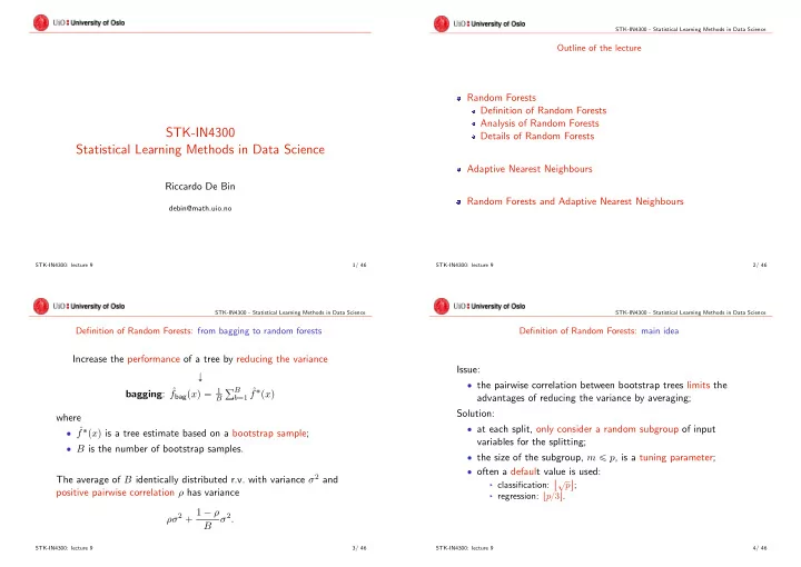
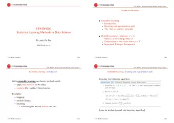
STK-IN4300 - Statistical Learning Methods in Data Science Outline of the lecture Random Forests Definition of Random Forests Analysis of Random Forests STK-IN4300 Details of Random Forests Statistical Learning Methods in Data Science Adaptive Nearest Neighbours Riccardo De Bin Random Forests and Adaptive Nearest Neighbours debin@math.uio.no STK-IN4300: lecture 9 1/ 46 STK-IN4300: lecture 9 2/ 46 STK-IN4300 - Statistical Learning Methods in Data Science STK-IN4300 - Statistical Learning Methods in Data Science Definition of Random Forests: from bagging to random forests Definition of Random Forests: main idea Increase the performance of a tree by reducing the variance Issue: Ó ‚ the pairwise correlation between bootstrap trees limits the bagging : ˆ b “ 1 ˆ f bag p x q “ 1 ř B f ˚ p x q advantages of reducing the variance by averaging; B Solution: where ‚ at each split, only consider a random subgroup of input ‚ ˆ f ˚ p x q is a tree estimate based on a bootstrap sample; variables for the splitting; ‚ B is the number of bootstrap samples. ‚ the size of the subgroup, m ď p , is a tuning parameter; ‚ often a default value is used: The average of B identically distributed r.v. with variance σ 2 and X ? p § classification: \ ; positive pairwise correlation ρ has variance § regression: t p { 3 u . ρσ 2 ` 1 ´ ρ σ 2 . B STK-IN4300: lecture 9 3/ 46 STK-IN4300: lecture 9 4/ 46

STK-IN4300 - Statistical Learning Methods in Data Science STK-IN4300 - Statistical Learning Methods in Data Science Definition of Random Forests: algorithm Definition of Random Forests: classification vs regression For b “ 1 to B : Depending on the problem, the prediction at a new point x : (a) Draw a bootstrap sample Z ˚ from the data; ‚ regression: ˆ ř B (b) Grow a random tree T b to the bootstrap data, by recursively f B rf p x q “ 1 b “ 1 T b p x ; Θ b q , B repeating steps (i), (ii), (iii) for each terminal node until the § where Θ b “ t R b , c b u characterizes the tree in terms of split minimum node size n min is reached: variables, cutpoints at each node and terminal node values; (i) randomly select m ď p variables; (ii) pick the best variable/split point only using the m selected ‚ classification: ˆ rf “ majority vote t ˆ C B C b p x ; Θ b qu B 1 , variables; § where ˆ (iii) split the node in two daughter nodes. C b p x ; Θ b q is the class prediction of the random-forest tree computed on the b -th bootstrap sample. The output is the ensemble of trees t T b u B b “ 1 . STK-IN4300: lecture 9 5/ 46 STK-IN4300: lecture 9 6/ 46 STK-IN4300 - Statistical Learning Methods in Data Science STK-IN4300 - Statistical Learning Methods in Data Science Definition of Random Forests: further tuning parameter n min Definition of Random Forests: further tuning parameter n min The step p b q of the algorithm claims that a tree must be grow until a specific number of terminal nodes, n min ; ‚ additional tuning parameter; ‚ Segal (2004) demonstrated some gains in the performance of the random forest when this parameter is tuned; ‚ Hastie et al. (2009) argued that it is not worth adding a tuning parameter, because the cost of growing the tree completely is small. STK-IN4300: lecture 9 7/ 46 STK-IN4300: lecture 9 8/ 46

STK-IN4300 - Statistical Learning Methods in Data Science STK-IN4300 - Statistical Learning Methods in Data Science Definition of Random Forests: more on the tuning parameters Definition of Random Forests: more on the tuning parameters In contrast, Hastie et al. (2009) showed that the default choice for the tuning parameter is not always the best. Consider the California Housing data: ‚ aggregate data of 20 . 460 neighbourhoods in California; ‚ response: median house value (in $100 . 000 ); ‚ eight numerical predictors (input): § MedInc : median income of the people living in the neighbour; § House : house density (number of houses); § AveOccup : average occupancy of the house; § longitude : longitude of the house; § latitude : latitude of the house; § AveRooms : average number of rooms per house; § AveBedrms : average number of bedrooms per house. STK-IN4300: lecture 9 9/ 46 STK-IN4300: lecture 9 10/ 46 STK-IN4300 - Statistical Learning Methods in Data Science STK-IN4300 - Statistical Learning Methods in Data Science Definition of Random Forests: more on the tuning parameters Analysis of Random Forests: estimator Consider the random forest estimator, Note that: B 1 ˆ ÿ f rf p x q “ lim T b p x ; Θ b q “ E Θ r T p x ; Θ qs , ‚ t 8 { 3 u “ 2 , but the results are better with m “ 6 ; B B Ñ8 b “ 1 ‚ the test error for the two random forests stabilizes at B “ 200 , no further improvements in considering more a regression problem and a square error loss. bootstrap samples; To make more explicit the dependence on the training sample Z , ‚ in contrast, the two boosting algorithms keep improving; the book rewrite ‚ in this case, boosting outperforms random forests. ˆ f rf p x q “ E Θ | Z r T p x ; Θ p Z qqs . STK-IN4300: lecture 9 11/ 46 STK-IN4300: lecture 9 12/ 46

STK-IN4300 - Statistical Learning Methods in Data Science STK-IN4300 - Statistical Learning Methods in Data Science Analysis of Random Forests: correlation Analysis of Random Forests: correlation Consider a single point x . Then, Var r ˆ f rf p x qs “ ρ p x q σ 2 p x q , Note: ‚ ρ p x q is NOT the average correlation between where: T b 1 p x ; Θ b 1 p Z “ z qq and T b 2 p x ; Θ b 2 p Z “ z qq , ‚ ρ is the sampling correlation between any pair of trees, b 1 ‰ b 2 “ 1 , . . . , B that form a random forest ensemble; ‚ ρ p x q is the theoretical correlation between a T b 1 p x ; Θ 1 p Z qq ρ p x q “ corr r T p x ; Θ 1 p Z qq , T p x ; Θ 2 p Z qqs and T b 2 p x ; Θ 2 p Z qq when drawing Z from the population and where Θ 1 p Z q and Θ 2 p Z q are a randomly drawn pair of drawing a pair of random trees; random forest trees grown to the randomly sampled Z ; ‚ ρ p x q is induced by the sampling distribution of Z and Θ . ‚ σ 2 p x q is the sampling variance of any single randomly drawn tree, σ 2 p x q “ V ar r T p x ; Θ 2 p Z qqs . STK-IN4300: lecture 9 13/ 46 STK-IN4300: lecture 9 14/ 46 STK-IN4300 - Statistical Learning Methods in Data Science STK-IN4300 - Statistical Learning Methods in Data Science Analysis of Random Forests: correlation Analysis of Random Forests: correlation Consider the following simulation model, 1 ÿ ? Y “ 50 X j ` ǫ 50 j “ 1 where X j , j “ 1 , . . . , 50 and ǫ are i.i.d. Gaussian. Generate: ‚ training sets: 500 training sets of 100 observations each; ‚ test sets: 600 sets of 1 observation each. STK-IN4300: lecture 9 15/ 46 STK-IN4300: lecture 9 16/ 46

STK-IN4300 - Statistical Learning Methods in Data Science STK-IN4300 - Statistical Learning Methods in Data Science Analysis of Random Forests: variance Analysis of Random Forests: variance Consider now the variance of the single tree, Var r T p x ; Θ p Z qqs . It can be decomposed as “ ‰ “ ‰ Var Θ ,Z r T p x ; Θ p Z qqs “ Var Z E Θ | Z r T p x ; Θ p Z qqs ` E Z Var Θ | Z r T p x ; Θ p Z qqs looooooooooomooooooooooon looooooooooooooomooooooooooooooon looooooooooooooomooooooooooooooon total variance within-Z variance Var Z ˆ f rf p x q where: ‚ Var Z ˆ f rf p x q : sampling variance of the random forest ensemble, § decreases with m decreasing; ‚ within-Z variance: variance resulting from the randomization, § increases with m decreasing; STK-IN4300: lecture 9 17/ 46 STK-IN4300: lecture 9 18/ 46 STK-IN4300 - Statistical Learning Methods in Data Science STK-IN4300 - Statistical Learning Methods in Data Science Analysis of Random Forests: variance Details of Random Forests: out of bag samples An important feature of random forests is its use of out-of-bag As in bagging, the bias is that of any individual tree, (OOB) samples: Bias p x q “ µ p x q ´ E Z r ˆ f rf p x qs , ‚ each tree is computed on a bootstrap sample; “ ‰ “ µ p x q ´ E Z E Θ | Z r T p x ; Θ p Z qqs ‚ some observations z i “ p x i , y i q are not included; ‚ compute the error by only averaging trees constructed on It is typically greater than the bias of an unpruned tree: bootstrap samples not containing z i Ñ OOB error. ‚ randomization; ‚ reduced sample space. ‚ OOB error is almost identical to N-fold cross-validation; General trend: larger m , smaller bias. ‚ random forests can be fit in one sequence. STK-IN4300: lecture 9 19/ 46 STK-IN4300: lecture 9 20/ 46