STK-IN4300 The bet on sparsity principle Statistical Learning - - PowerPoint PPT Presentation

STK-IN4300 Statistical Learning Methods in Data Science

Riccardo De Bin

debin@math.uio.no

STK-IN4300: lecture 12 1/ 43 STK-IN4300 - Statistical Learning Methods in Data Science

Outline of the lecture

Ensemble Learning Introduction Boosting and regularization path The “bet on sparsity” principle High-Dimensional Problems: p " N When p is much larger than N Computational short-cuts when p " N Supervised Principal Component

STK-IN4300: lecture 12 2/ 43 STK-IN4300 - Statistical Learning Methods in Data Science

Ensemble Learning: introduction

With ensemble learning we denote methods which: ‚ apply base learners to the data; ‚ combine the results of these learner. Examples: ‚ bagging; ‚ random forests; ‚ boosting,

§ in boosting the learners evolves over time. STK-IN4300: lecture 12 3/ 43 STK-IN4300 - Statistical Learning Methods in Data Science

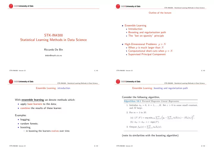
Ensemble Learning: boosting and regularization path

Consider the following algorithm, (note its similarities with the boosting algorithm)

STK-IN4300: lecture 12 4/ 43

STK-IN4300 - Statistical Learning Methods in Data Science

Ensemble Learning: boosting and regularization path

In comparison with lasso: ‚ initialization (˘ αk “ 0, k “ 1, . . . , K) Ð Ñ λ “ 8; ‚ for small values of M:

§ some ˘

αk are not updated Ð Ñ coefficients “forced” to be 0;

§ ˘

αr0s

k

ď ˘ αrMs

k

ď ˘ αr8s

k

Ð Ñ shrinkage;

§ M inversely related to λ;

‚ for M large enough (M “ 8 in boosting) and K ă N, ˘ αrMs

k

“ ˆ αLS Ð Ñ λ “ 0

STK-IN4300: lecture 12 5/ 43 STK-IN4300 - Statistical Learning Methods in Data Science

Ensemble Learning: boosting and regularization path

STK-IN4300: lecture 12 6/ 43 STK-IN4300 - Statistical Learning Methods in Data Science

Ensemble Learning: boosting and regularization path

If ‚ all the basis learners TK are mutually uncorrelated, then ‚ for ε Ñ 0 and M Ñ 8, such that εM Ñ t, Algorithm 16.1 gives the lasso solutions with t “ ř

k |αk|.

In general component-wise boosting and lasso do not provide the same solution: ‚ in practice, often similar in terms of prediction; ‚ for ε (ν) Ñ 0 boosting (and forward stagewise in general) tends to the path of the least angle regression algorithm; ‚ lasso can also be seen as a special case of least angle.

STK-IN4300: lecture 12 7/ 43 STK-IN4300 - Statistical Learning Methods in Data Science

Ensemble Learning: boosting and regularization path

Consider 1000 Gaussian distributed variables: ‚ strongly correlated (ρ “ 0.95) in blocks of 20; ‚ uncorrelated blocks; ‚ one variable with effect on the outcome for each block; ‚ effects generated from a standard Gaussian. Moreover: ‚ added Gaussian noise; ‚ noise-to-signal ratio = 0.72.

STK-IN4300: lecture 12 8/ 43

STK-IN4300 - Statistical Learning Methods in Data Science

Ensemble Learning: boosting and regularization path

STK-IN4300: lecture 12 9/ 43 STK-IN4300 - Statistical Learning Methods in Data Science

Ensemble Learning: boosting and regularization path

STK-IN4300: lecture 12 10/ 43 STK-IN4300 - Statistical Learning Methods in Data Science

Ensemble Learning: the “bet on sparsity” principle

We consider: ‚ L1-type of penalty (shrinkage, variable selection); ‚ L2-type of penalty (shrinkage, computationally easy); ‚ boosting’s stagewise forward strategy minimizes something close to a L1 penalized loss function; ‚ step-by-step minimization. Can we characterize situations where one is preferable to the other?

STK-IN4300: lecture 12 11/ 43 STK-IN4300 - Statistical Learning Methods in Data Science

Ensemble Learning: the “bet on sparsity” principle

Consider the following framework: ‚ 50 observations; ‚ 300 independent Gaussian variables. Three scenarios: ‚ all 300 variables are relevant; ‚ only 10 out of 300 variables are relevant; ‚ 30 out of 300 variables are relevant. Outcome: ‚ regression (added standard Gaussian noise); ‚ classification (from an inverse-logit transformation of the linear predictor)

STK-IN4300: lecture 12 12/ 43

STK-IN4300 - Statistical Learning Methods in Data Science

Ensemble Learning: the “bet on sparsity” principle

STK-IN4300: lecture 12 13/ 43 STK-IN4300 - Statistical Learning Methods in Data Science

Ensemble Learning: the “bet on sparsity” principle

STK-IN4300: lecture 12 14/ 43 STK-IN4300 - Statistical Learning Methods in Data Science

Ensemble Learning: the “bet on sparsity” principle

STK-IN4300: lecture 12 15/ 43 STK-IN4300 - Statistical Learning Methods in Data Science

Ensemble Learning: the “bet on sparsity” principle

This means that: ‚ lasso performs better than ridge in sparse contexts; ‚ ridge gives better results if there are several relevant variables with small effects; ‚ anyway, in the dense case, the model does not explain a lot,

§ not enough data to estimate correctly several coefficients;

Ó “bet on sparsity” “ “use a procedure that does well in sparse problems, since no procedure does well in dense problems”

STK-IN4300: lecture 12 16/ 43

STK-IN4300 - Statistical Learning Methods in Data Science

Ensemble Learning: the “bet on sparsity” principle

The degree of sparseness depends on: ‚ the unknown mechanism generating the data;

§ it depends on the number of relevant variables;

‚ size of the training set;

§ larger sizes allow estimating denser models;

‚ noise-to-signal ratio;

§ smaller NSR Ñ denser models (same as before);

‚ size of the dictionary;

§ more base learners, potentially sparser models. STK-IN4300: lecture 12 17/ 43 STK-IN4300 - Statistical Learning Methods in Data Science

High-Dimensional Problems: when p is much larger than N

The case p " N (number of variable much larger than the number

• f observations):

‚ very important in current applications,

§ e.g., in a common genetic study, p « 23000, N « 100;

‚ concerns about high variance and overfitting; ‚ highly regularized approaches are common:

§ lasso; § ridge; § boosting; § elastic-net; § . . . STK-IN4300: lecture 12 18/ 43 STK-IN4300 - Statistical Learning Methods in Data Science

High-Dimensional Problems: when p is much larger than N

Consider the following example: ‚ N “ 100; ‚ p variables from standard Gaussians with ρ “ 0.2, (i) p “ 20 (ii) p “ 100 (iii) p “ 1000. ‚ response from Y “ řp

j“1 Xjβj ` σǫ;

‚ signal to noise ratio VarrEpY |Xqs{σ2 “ 2; ‚ true β from a standard Gaussian;

STK-IN4300: lecture 12 19/ 43 STK-IN4300 - Statistical Learning Methods in Data Science

High-Dimensional Problems: when p is much larger than N

As a consequence, averaging over 100 replications: ‚ p0, the number of significant β (i.e., β : |ˆ β{ ˆ se| ą 2) (i) p0 “ 9 (ii) p0 “ 33 (iii) p0 “ 331. Consider 3 values of the penalty λ: ‚ λ “ 0.001, which corresponds to (i) d.o.f. “ 20 (ii) d.o.f. “ 99 (iii) d.o.f. “ 99; ‚ λ “ 100, which corresponds to (i) d.o.f. “ 9 (ii) d.o.f. “ 35 (iii) d.o.f. “ 87; ‚ λ “ 1000, which corresponds to (i) d.o.f. “ 2 (ii) d.o.f. “ 7 (iii) d.o.f. “ 43.

STK-IN4300: lecture 12 20/ 43

STK-IN4300 - Statistical Learning Methods in Data Science

High-Dimensional Problems: when p is much larger than N

STK-IN4300: lecture 12 21/ 43 STK-IN4300 - Statistical Learning Methods in Data Science

High-Dimensional Problems: when p is much larger than N

Remarks: ‚ with p “ 20, ridge regression can find the relevant variables;

§ the covariance matrix can be estimated;

‚ moderate shrinkage works better in the middle case, in which we can find some non-zero effects; ‚ with p “ 1000, there is no hope to find the relevant variables, and it is better to shrink down everything;

§ no possibility to estimate the covariance matrix. STK-IN4300: lecture 12 22/ 43 STK-IN4300 - Statistical Learning Methods in Data Science

High-Dimensional Problems: computational short-cuts when p " N

Consider the single-value decomposition of X, X “ UDV T “ RV T Where ‚ V is a p ˆ N matrix with orthonormal columns; ‚ U is a N ˆ N orthonormal matrix; ‚ D is a diagonal matrix with elements d1 ě d2 ě ¨ ¨ ¨ ě dN ě 0; ‚ R is a N ˆ N with rows rT

i .

STK-IN4300: lecture 12 23/ 43 STK-IN4300 - Statistical Learning Methods in Data Science

High-Dimensional Problems: computational short-cuts when p " N

Theorem (Hastie et al., 2009, page 660): Let f˚priq “ θ0 ` rT

i θ and consider the optimization problems:

pˆ β0, ˆ βq “ argminβ0,βPRp

N

ÿ

i“1

Lpyi, β0 ` xiβq ` λβT β; pˆ θ0, ˆ θq “ argminθ0,θPRN

N

ÿ

i“1

Lpyi, θ0 ` rT

i θq ` λθT θ.

Then β0 “ θ0 and ˆ β “ V ˆ θ.

STK-IN4300: lecture 12 24/ 43

STK-IN4300 - Statistical Learning Methods in Data Science

High-Dimensional Problems: computational short-cuts when p " N

Note: ‚ we can replace the p-dim vectors xi with the N-dim vectors ri; ‚ same penalization, but with way fewer predictors; ‚ the N-dimensional solution ˆ θ is transformed back to the p-dimensional ˆ β by simple matrix multiplication; ‚ it only works for linear models; ‚ it only works for quadratic penalties. ‚ a Opp3q problem is reduced to a Opp2Nq problem;

§ relevant for p ą N. STK-IN4300: lecture 12 25/ 43 STK-IN4300 - Statistical Learning Methods in Data Science

High-Dimensional Problems: computational short-cuts when p " N

Example (ridge regression): Consider the estimate of a ridge regression, ˆ β “ pXT X ` λIq´1XT y. Replacing X with RV T , we obtain ˆ β “ V pRT R ` λIq´1RT y, i.e., ˆ β “ V ˆ θ, where ˆ θ “ pRT R ` λIq´1RT y.

STK-IN4300: lecture 12 26/ 43 STK-IN4300 - Statistical Learning Methods in Data Science

High-Dimensional Problems: computational short-cuts when p " N

Note: ‚ it cannot be applied to lasso; ‚ the short-cut is particularly relevant for finding the best λ via cross-validation; ‚ it can be shown that one need to construct R only once,

§ use the same R for each of the CV-folds. STK-IN4300: lecture 12 27/ 43 STK-IN4300 - Statistical Learning Methods in Data Science

High-Dimensional Problems: supervised principal component

STK-IN4300: lecture 12 28/ 43

STK-IN4300 - Statistical Learning Methods in Data Science

High-Dimensional Problems: supervised principal component

Note: ‚ in the first step, the variables univariately most associated with the outcome are selected:

§ the measure depends on the nature of the outcome; § include all associations larger than a threshold θ; § may include highly correlated variables.

‚ in step 2, perform PCR on the reduced variable space:

§ use the first m components; § assure shrinkage.

‚ both θ and m must be computed by cross-validation:

§ 2-dimension tuning parameter. STK-IN4300: lecture 12 29/ 43 STK-IN4300 - Statistical Learning Methods in Data Science

High-Dimensional Problems: supervised principal component

Example (survival analysis with microarray data): ‚ data from Rosenwald et al. (2002); ‚ input: 7399 gene expressions of 240 patients; ‚ response: survival time (potentially right censored); ‚ divided in a training (160 patients) and (80) test set.

STK-IN4300: lecture 12 30/ 43 STK-IN4300 - Statistical Learning Methods in Data Science

High-Dimensional Problems: supervised principal component

STK-IN4300: lecture 12 31/ 43 STK-IN4300 - Statistical Learning Methods in Data Science

High-Dimensional Problems: supervised principal component

STK-IN4300: lecture 12 32/ 43

STK-IN4300 - Statistical Learning Methods in Data Science

High-Dimensional Problems: supervised principal component

STK-IN4300: lecture 12 33/ 43 STK-IN4300 - Statistical Learning Methods in Data Science

High-Dimensional Problems: supervised principal component

STK-IN4300: lecture 12 34/ 43 STK-IN4300 - Statistical Learning Methods in Data Science

High-Dimensional Problems: supervised principal component

STK-IN4300: lecture 12 35/ 43 STK-IN4300 - Statistical Learning Methods in Data Science

High-Dimensional Problems: supervised-PC and latent-variable modelling

Consider a latent-variable model, Y “ β0 ` β1U ` ǫ where Xj “ α0j ` α1jU ` ǫj if j P P ‚ ǫ and ǫj have mean 0 and they are independent of the other variables in their respective models; ‚ Xj are independent of U if j R P.

STK-IN4300: lecture 12 36/ 43

STK-IN4300 - Statistical Learning Methods in Data Science

High-Dimensional Problems: supervised-PC and latent-variable modelling

Supervised-PC can be seen as a method to fit this kind of model: ‚ step 1: identify the j P P;

§ on average β1 is not zero only if α1j ‰ 0;

‚ step 2a: estimate α0j and α1j

§ natural if ǫj „ Np0; σ2q;

‚ step 2b: estimate β0 and β1 (fit the model).

STK-IN4300: lecture 12 37/ 43 STK-IN4300 - Statistical Learning Methods in Data Science

High-Dimensional Problems: supervised-PC and partial least square

Supervised-PC versus partial least square: ‚ both aim at considering both large variation and correlation with the outcome; ‚ supervised-PC removes those which are not relevant; ‚ partial least square downgrades them Ó “thresholded PLS”:

§ apply PLS on only the variables selected by supervised-PC. STK-IN4300: lecture 12 38/ 43 STK-IN4300 - Statistical Learning Methods in Data Science

High-Dimensional Problems: supervised-PC and partial least square

Thresholded PLS can be seen as a noisy version of supervised-PC, ‚ first PLS variate, z “ ř

jPPxy, xjyxj;

‚ supervised principal component direction, u “ 1

d2

ř

jPPxy, xjyxj.

Set p1 “ |P|. It can be shown (Bair & Tibshirani, 2004) that, for N, p1, p Ñ 8, s.t. p1{N Ñ 0 z “ u ` Opp1q ˆ u “ u ` Opp a p1{Nq where u is the true latent variable.

STK-IN4300: lecture 12 39/ 43 STK-IN4300 - Statistical Learning Methods in Data Science

High-Dimensional Problems: supervised-PC and partial least square

STK-IN4300: lecture 12 40/ 43

STK-IN4300 - Statistical Learning Methods in Data Science

High-Dimensional Problems: pre-conditioning

Supervised-PC can also be used to improve lasso performance, through pre-conditioning ‚ compute ˆ yi the supervised-PC prediction for each observation; ‚ apply lasso using ˆ yi instead of yi as outcome;

§ using all variables, not only those selected by supervised-PC.

The idea is to remove the noise, so lasso is not affected by the large number of noisy variables.

STK-IN4300: lecture 12 41/ 43 STK-IN4300 - Statistical Learning Methods in Data Science

High-Dimensional Problems: pre-conditioning

STK-IN4300: lecture 12 42/ 43 STK-IN4300 - Statistical Learning Methods in Data Science

References I

Bair, E. & Tibshirani, R. (2004). Semi-supervised methods to predict patient survival from gene expression data. PLoS Biology 2, e108. Hastie, T., Tibshirani, R. & Friedman, J. (2009). The Elements of Statistical Learning: Data Mining, Inference and Prediction (2nd Edition). Springer, New York. Rosenwald, A., Wright, G., Chan, W. C., Connors, J. M., Campo, E., Fisher, R. I., Gascoyne, R. D., Muller-Hermelink, H. K., Smeland, E. B., Giltnane, J. M. et al. (2002). The use of molecular profiling to predict survival after chemotherapy for diffuse large-b-cell

• lymphoma. New England Journal of Medicine 346, 1937–1947.

STK-IN4300: lecture 12 43/ 43