
SLIDE 1
Segmentation & Custering Disclaimer: Many slides have been - - PowerPoint PPT Presentation
Segmentation & Custering Disclaimer: Many slides have been borrowed from Devi Parikh and Kristen Grauman, who may have borrowed some of them from others. Any time a slide did not already have a credit on it, I have credited it to Kristen. So
2
Disclaimer: Many slides have been borrowed from Devi Parikh and Kristen Grauman, who may have borrowed some of them from
are inaccurate.
3
4
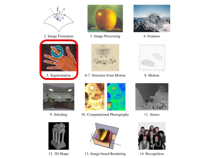
5
Slide credit: Kristen Grauman
[Figure by J. Shi] [http://poseidon.csd.auth.gr/LAB_RESEARCH/Latest/imgs/S peakDepVidIndex_img2.jpg]
Determine image regions Group video frames into shots Fg / Bg
[Figure by Wang & Suter]
Object-level grouping Figure-ground
[Figure by Grauman & Darrell]
6
Slide credit: Kristen Grauman
7
Slide credit: Kristen Grauman
8
Slide credit: Kristen Grauman
9
Slide credit: Kristen Grauman
10
11
12
13
Slide credit: Kristen Grauman
14
Slide credit: Devi Parikh Figure 14.4 from Forsyth and Ponce
15
Slide credit: Devi Parikh
http://chicagoist.com/attachments/chicagoist_alicia/GEESE.jpg, http://wwwdelivery.superstock.com/WI/223/1532/PreviewComp/SuperStock_1532R-0831.jpg
16
Kristen Grauman
http://seedmagazine.com/news/2006/10/beauty_is_in_the_processingtim.php
17
Slide credit: Kristen Grauman
Image credit: Arthus-Bertrand (via F. Durand)
18
Slide credit: Kristen Grauman
http://www.capital.edu/Resources/Images/outside6_035.jpg
19
Slide credit: Kristen Grauman
In Vision, D. Marr, 1982
20
Slide credit: Kristen Grauman
21
Slide credit: Kristen Grauman
22
Slide credit: Kristen Grauman
23
24
Slide credit: Kristen Grauman
25
Slide credit: Kristen Grauman
26
Slide credit: Kristen Grauman
27
Slide credit: Kristen Grauman
28
Slide credit: Kristen Grauman
29
Slide credit: Kristen Grauman
30
image human segmentation
Source: Lana Lazebnik
31
Source: Lana Lazebnik
32
black pixels gray pixels white pixels
Kristen Grauman 33
Kristen Grauman 34
Kristen Grauman 35
190 255
intensity
Kristen Grauman 36
Kristen Grauman 37
Source: Steve Seitz
38
39
Slide credit: Kristen Grauman
labeled by cluster center’s intensity
Kristen Grauman 40
41
Slide credit: Kristen Grauman
K=2 K=3
quantization of the feature space; segmentation label map
42
Slide credit: Kristen Grauman
R=255 G=200 B=250 R=245 G=220 B=248 R=15 G=189 B=2 R=3 G=12 B=2 R G B
Kristen Grauman 43
Kristen Grauman 44
X
Y Intensity Both regions are black, but if we also include position (x,y), then we could group the two into distinct segments; way to encode both similarity & proximity.
Kristen Grauman 45
46
Slide credit: Kristen Grauman
F24
F2
F1
Filter bank
47
Slide credit: Kristen Grauman
Malik, Belongie, Leung and Shi. IJCV 2001.
Texton map Image
Adapted from Lana Lazebnik
Texton index Texton index Count Count Count Texton index
48
Kristen Grauman 49
Kristen Grauman 50
51
52
Slide credit: Kristen Grauman
53
Slide credit: Kristen Grauman
Search window Center of mass Mean Shift vector
Slide by Y. Ukrainitz & B. Sarel
54
Search window Center of mass Mean Shift vector
Slide by Y. Ukrainitz & B. Sarel
55
Search window Center of mass Mean Shift vector
Slide by Y. Ukrainitz & B. Sarel
56
Search window Center of mass Mean Shift vector
Slide by Y. Ukrainitz & B. Sarel
57
Search window Center of mass Mean Shift vector
Slide by Y. Ukrainitz & B. Sarel
58
Search window Center of mass Mean Shift vector
Slide by Y. Ukrainitz & B. Sarel
59
Search window Center of mass
Slide by Y. Ukrainitz & B. Sarel
60
Slide by Y. Ukrainitz & B. Sarel
61
62
Slide credit: Kristen Grauman
http://www.caip.rutgers.edu/~comanici/MSPAMI/msPamiResults.html
63
Slide credit: Kristen Grauman
64
Slide credit: Kristen Grauman
Kristen Grauman
65
66
q
– similarity is inversely proportional to difference (color+position…) p wpq
Source: Steve Seitz 67
Kristen Grauman 68
Feature dimension 1 Feature dimension 2
Kristen Grauman
69
for i=1:N for j=1:N D(i,j) = ||xi- xj||2 end end
0.24 0.01 0.47 D(1,:)= D ( : , 1 ) = 0.24 0.01 0.47 (0)
Kristen Grauman
70
for i=1:N for j=1:N D(i,j) = ||xi- xj||2 end end
D(1,:)= D ( : , 1 ) = 0.24 0.01 0.47 (0) 0.15 0.24 0.29 (0) 0.29 0.15 0.24
Kristen Grauman
71
for i=1:N for j=1:N D(i,j) = ||xi- xj||2 end end
N x N matrix
Kristen Grauman
72
for i=1:N for j=1:N D(i,j) = ||xi- xj||2 end end for i=1:N for j=i+1:N A(i,j) = exp(-1/(2*σ^2)*||xi- xj||2); A(j,i) = A(i,j); end end
Kristen Grauman
73
Kristen Grauman
74
Kristen Grauman
75
σ=.1 σ=.2 σ=1 σ=.2
76
Slide credit: Kristen Grauman
, -.2
2}
Points x1…x10 Points x31…x40
x1 . . . x40 x1 . . . x40
77
Slide credit: Kristen Grauman
σ=.1 σ=.2 σ=1 Data points Affinity matrices Points x1…x10 Points x31…x40
, -.2
2}
Kristen Grauman
78
Source: Steve Seitz
q p wpq
79
Source: Steve Seitz
Î Î
B q A p q p
, ,
80
[Shi & Malik, 2000 PAMI]
81
Slide credit: Kristen Grauman
assoc(A,V) = sum of weights of all edges that touch A
with high weights, and few edges of low weight between them
generalized eigenvalue problem.
Source: Steve Seitz
82
83
Slide credit: Kristen Grauman
84
Slide credit: Kristen Grauman
– Dense, highly connected graphs à many affinity computations – Solving eigenvalue problem
Kristen Grauman 85
86
Multiple segmentations
Slide credit: Lana Lazebnik 87
Slide credit: Lana Lazebnik
2006.
88
2006. Normalized cuts Top-down segmentation
Slide credit: Lana Lazebnik 89
90
Slide credit: Kristen Grauman
91
92
93