Stefano Cristiani Stefano Cristiani INAF- INAF -Observatory of - - PowerPoint PPT Presentation

stefano cristiani stefano cristiani inaf inaf observatory
SMART_READER_LITE
LIVE PREVIEW

Stefano Cristiani Stefano Cristiani INAF- INAF -Observatory of - - PowerPoint PPT Presentation

Stefano Cristiani Stefano Cristiani INAF- INAF -Observatory of Trieste Observatory of Trieste for the CODEX team for the CODEX team 1 Relativistic Big Bang Cosmology Universal Expansion Relativistic Big Bang Cosmology Expansion


slide-1
SLIDE 1

1

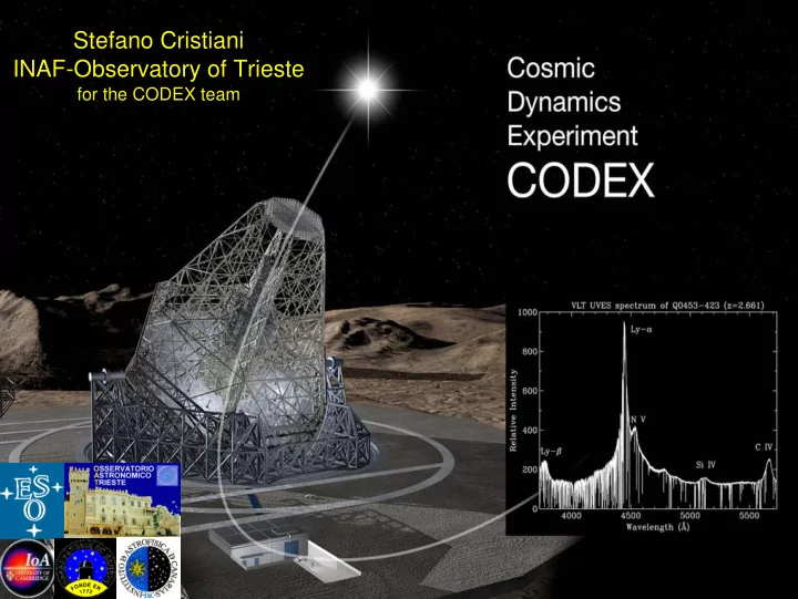
Stefano Cristiani Stefano Cristiani INAF INAF-

  • Observatory of Trieste

Observatory of Trieste

for the CODEX team for the CODEX team

slide-2
SLIDE 2

Relativistic Big Bang Cosmology

Universal Expansion

slide-3
SLIDE 3

Relativistic Big Bang Cosmology

Abundance

  • f light

elements Structure formation Cosmic Microwave Background Expansion

slide-4
SLIDE 4

Which of the solutions of the Friedmann equation corresponds to reality?

Or in other words: What is the stress-energy tensor of the universe? For each mass/energy component i, what is Ωi, wi? How can these be measured?

Dynamics Geometry Clustering (the universe is not homogeneous on small scales!)

Equation of state parameter Density parameter Both determined by gravity in GR

slide-5
SLIDE 5

Which of the solutions of the Friedmann equation corresponds to reality?

Answers have already been provided by:

  • Cosmic Microwave

Cosmic Microwave Background Background

  • Supernovae type Ia

Supernovae type Ia

  • Large scale structure of

Large scale structure of galaxies and intergalactic galaxies and intergalactic medium medium

  • Galaxy clusters

Galaxy clusters

  • Weak lensing

Weak lensing

Tegmark et al. (2004)

slide-6
SLIDE 6

With the assumptions of homogeneity and isotropy, the concordance model finds a FRW metric with a non zero cosmological constant

Standard Model

We do not know what We do not know what ρ ρλ

λ is and

is and how it evolves. how it evolves. Dynamics has never been Dynamics has never been measured measured. . All other experiments, such as All other experiments, such as High Z High Z SNae SNae search and CMB search and CMB measure measure geometry geometry: : dimming of magnitudes and dimming of magnitudes and scattering at the recombination scattering at the recombination surface and surface and clustering clustering (growth of (growth of structure). structure). Measurements of the Measurements of the dynamics of the Universe dynamics of the Universe can be compared to basic can be compared to basic experiments such as the test experiments such as the test

  • f the equivalence principle
  • f the equivalence principle

Inertial Inertial -

  • Gravitational

Gravitational mass… mass…

slide-7
SLIDE 7

Can we measure the history

  • f the expansion directly?

a(t) t

Goal is to measure or reconstruct the unknown function a(t).

slide-8
SLIDE 8

Can we measure the history

  • f the expansion directly?

a(t) t

H

Δt Δa Yes: Measure a(z), da/dt(z) → a(t) Need to measure H(z) using the dynamics!

slide-9
SLIDE 9

Can we measure the history

  • f the expansion directly?

a(t) t

H

Δt Δa Yes: Measure a(z), da/dt(z) → a(t) Need to measure H(z) using the dynamics!

slide-10
SLIDE 10

Can we measure the history

  • f the expansion directly?

a(t) t

H

Δt Δa Yes: Measure a(z), da/dt(z) → a(t) Need to measure H(z) using the dynamics!

slide-11
SLIDE 11

a(t0 + Δt0) a(t0) a(te) a(te + Δte) a(t) t te te + Δte t0 t0 + Δt0

H(z) H0

Measuring H(z)

z t 0 dz dt 0 1 z H 0 H z

z(t0 + Δt0) - z(t0)

Δt0

(te)

slide-12
SLIDE 12

The change in sign is the signature of the non zero cosmological constant

The Signal is SMALL!

slide-13
SLIDE 13

How to Measure this signal?

Masers : in principle very good candidates: lines are very narrow and measurements accurate: however they sit at the center of huge potential wells: large peculiar accelerations , larger than the Cosmic Signal are expected Molecular Lines with ALMA: as for Masers, local motions of the emitters are real killers. Few radio galaxies so far observed show variability at a level much higher than the signal we should like to detect Ly Lyα α forest forest: : Absorption from the many intervening lines in front of high-z QSOs are the most promising candidates. Simulations,

  • bservations and analysis all concur in indicating that Lyα forest

and associated metal lines are produced by systems sitting in a warm IGM following beautifully the Hubble flow !

slide-14
SLIDE 14

The Lyman Forest The Lyman Forest Today and … Today and … … years after … years after

slide-15
SLIDE 15

Observing dz/dt in the Ly-α Forest

slide-16
SLIDE 16

Observing dz/dt in the Ly-α Forest

slide-17
SLIDE 17

Observing dz/dt in the Ly-α Forest

Δt = 106 years!

slide-18
SLIDE 18

Observing dz/dt in the Ly-α Forest

Δt = 10 years: ΔTrans ~ 10-6

slide-19
SLIDE 19
slide-20
SLIDE 20

The European Extremely Large Telescope

42 m aperture

~900 1.45m mirror segments NIR/optical First light 2017?

See

http://www.eso.org/public/ astronomy/projects/e- elt.html

for details

slide-21
SLIDE 21

The HARPS Experience

O-C < 80 cm/sec Th-Th < 10 cm/sec

slide-22
SLIDE 22

HARPS: it is possible!

  • Exoplanets (HARPS)

long term accuracy 1m/s, short term (hours) 0.1m/s (and largely understood)

  • ELT !! LOT OF

PHOTONS (we need them!!)

slide-23
SLIDE 23

The Team

ESO: G. Avila, B. Delabre, H. Dekker, S. D’Odorico, J. Liske, A.Manescau, L. Pasquini, P. Shaver Observatoire Geneve : M.Dessauges-Zavadsky, M. Fleury, C. Lovis, M. Mayor, D.Megevand, F. Pepe, D. Queloz, S. Udry INAF-Trieste P. Bonifacio, S. Cristiani, I.Coretti, V. D’Odorico, P. Di Marcantonio, P. Molaro, P.Santin, E.Vanzella, M.Viel Institute of Astronomy Cambridge: M. Haehnelt, R.Carswell, M. Murphy IAC: R. García López, J.M.Herreros, G.Israelian, A.Manchado, E. Martin,

  • J. Perez, R. Rebolo, J. Sanchez Béjar, M.R.Zapatero

OTHERS: F. Bouchy (Marseille), S. Borgani (DAUT-Ts), A. Grazian (INAF-OAR), S. Levshakov (St-Petersburg), L. Moscardini (UNIBo),

  • S. Zucker (Tel Aviv), P.Spano (INAF-Brear), T. Wilklind (ESA),

F.Zerbi (INAF-Brera)

CO COsmic D Dynamics EX EXperiment

slide-24
SLIDE 24

What S/N do we need to detect dz/dt?

What radial velocity accuracy can we achieve using the Lyα forest? How does the sensitivity depend on redshift?

Real absorption line lists: derived from high- resolution, high-S/N UVES/VLT spectra

(Kim, Cristiani & D’Odorico. 2002).

slide-25
SLIDE 25

What S/N do we need to detect dz/dt?

What radial velocity accuracy can we achieve using the Lyα forest? How does the sensitivity depend on redshift?

where the S/N is per 0.0125 Å pixel (4 pixel per resolution element at R = 100 000). Assumed 2 epochs

v

2 S N 1450

1

N QSO 30

1 2

1 z QSO 5

1.7 0.9

cm s

Liske et al. 2007

2370

slide-26
SLIDE 26

A simulated measurement

~2 nights ~2 nights /month over /month over 15 years will 15 years will deliver any deliver any

  • ne
  • ne of these
  • f these

sets of sets of points. points.

Not observable from the ground!

slide-27
SLIDE 27

Are there enough photons in the sky?

Yes! 20 known Yes! 20 known QSOs QSOs with with 2< z < 5 are bright enough 2< z < 5 are bright enough to achieve a radial velocity to achieve a radial velocity accuracy of 3 cm/s with accuracy of 3 cm/s with 3200 hours on a 42 3200 hours on a 42-

  • m ELT.

m ELT.

and more will come (SDSS, GAIA...)

slide-28
SLIDE 28

CODEX – The Instrument

Basic spectrograph requirements (wish list):

Spectral range: Want to span as large a redshift range as possible. Beyond z ~ 4-5 the Lyα forest “saturates” . Cannot observe below ~300 nm from ground. Ideal range = 300 – 680 nm. Resolution: Lyα lines have typical widths of 20-30 km/s. R = 50,000 would suffice. But higher resolution is required by metal lines and wavelength calibration. R ~ 150,000

Long term stability: ~1 cm/s over ~10 years.

slide-29
SLIDE 29

Camera Light enters here Echelle mosaic 20x160 cm

Delabre & Dekker (ESO)

Cross-disperser Anamorphic collimator Pupil slicer VPHG

Cross disperser 10 x VPHG 1500 l/mm 15 x 15 cm Camera 10 x F/1.4-2.8 CCD 10 x ~8K x 8K (15 µm pixels) 360 Mpix or 810 cm2

Main disperser 5 x R4 echelle 42 l/mm 160 x 20 cm

slide-30
SLIDE 30

CODEX underground laboratory floor plan

Underground hall 20x30x8 m 1K Instrument room 10x20x5 m 0.1K Control room and auxiliary equipment 1K Optical bench and detector 0.001K Instrument tanks 2.5x4 m Instrument tanks 2.5x4 m 0.01K 0.01K

slide-31
SLIDE 31

Potential Problems

Changes in absorber ionisation structure (e.g. winds in the IGM) QSO continuum variability Weak lensing Wavelength calibration Wavelength calibration Fibre throughput Heliocentric correction (GAIA...) Temperature control Guiding accuracy

None of these are currently believed to be show-stoppers.

slide-32
SLIDE 32

Wavelength Calibration

Classical method: ThAr comparison spectra.

Problems: Long-term stability? Low line density in some parts of the optical spectrum.

Alternative: Observe object spectrum through an iodine

  • cell. Problems: Long-term stability? Loss of flux

System pursued for CODEX:

Optical or NIR laser producing a train of monochromatic femtosecond light pulses. Pulse repetition rate is controlled by an atomic clock. Produces a spectrum of evenly spaced δ-functions (frequency comb) whose absolute wavelengths are known to a precision limited only by the atomic clock. Current problem: comb is too dense, would need R=600,000 to resolve it.

slide-33
SLIDE 33

Laser Comb

Train of femtosecond light pulses

  • Frequency

comb Zero offset and line spacing known with absolute precision (limit = atomic clock.)

Thomas Udem (MPQ)

slide-34
SLIDE 34

Immediate Science (first epoch data)

  • Cosmological variation of the fine structure

Cosmological variation of the fine structure constant constant

– Accuracy in Δα/α ~ 10-8

slide-35
SLIDE 35

Immediate Science (first epoch data)

Terrestrial extra Terrestrial extra-

  • solar

solar planets planets

  • Radial velocity follow-up
  • f earth-mass planet

candidates discovered through other techniques(astrometry, transits). Different environments and formation histories (GCs, DGs)

  • Difficulty: “seeing” the

planet through the noise of stellar activity

slide-36
SLIDE 36

Immediate Science

(things we can do with the first epoch data)

Cosmological variation of the fine structure constant

Accuracy in Δα/α ~ 10-8

Terrestrial extra-solar planets

Radial velocity follow-up of earth-mass planet candidates discovered through other techniques(astrometry, transits). Different environments and formation histories (GCs, DGs)

Primordial Primordial nucleosynthesis nucleosynthesis Primordial abundances of D, 7Li, 6Li / 7Li Primordial abundances of D, 7Li, 6Li / 7Li

slide-37
SLIDE 37

One giant leap from HARPS (3.6m)?

Need for a prototype Better… a precursor precursor ESPRESSO ESPRESSO E Echelle S Spectrograph for PRE PREcision S Super S Stable O Observations @ the ESO VLT – possibly @ the incoherently combined focus of the 4 UTs

slide-38
SLIDE 38

ESPRESSO ESPRESSO – – The Instrument The Instrument

Radial velocity accuracy: Radial velocity accuracy: 10 cm/s at any time scale from 20 s up to 30 y (1 cm/s from 30 s up to 30 y) Spectral coverage Spectral coverage: (350) 370-686 (720) nm corresponding to z (1.89) 2.04-4.64 (4.92) in the Lya forest Spectral Resolution: Spectral Resolution: 1-UT mode R = 150,000 (180,000) 4-UT mode A R > 45,000 4-UT mode B R > 90,000 Spectral sampling: Spectral sampling: 3.5 pixels/FWHM (4 pixels/FWHM) Feed: Feed: 1 object fiber, 1 reference and/or sky fiber Total aperture on the sky: Total aperture on the sky: 1.2 > FOV > 0.9 arcsec Total detection efficiency: Total detection efficiency: at least 18% (at peak wavelength and at blaze maximum) and not less than 9% (0.8 arsec DIMM)

slide-39
SLIDE 39

ESPRESSO – Science +

Multiple LOS expansion-collapse in the cosmic web winds

Rauch, Becker, Viel et al. 2006

slide-40
SLIDE 40

Summary

Performing a direct and purely dynamical measurement of the expansion history of the universe is a fundamental physics experiment. A direct and “natural” way to perform this measurement is by

  • bserving the change of redshift of cosmological sources as a

function of time, which is a direct signal of the de/acceleration

  • f the universe's expansion.

In principle the experiment does not involve or rely on any astrophysics (such as the [unknown] evolution of the sources used). The signal is from a different cosmic epoch compared to CMB or SNe Ia data.

A high-resolution optical spectrograph with exceptional stability

  • n an ELT (> ~40 m) is capable of detecting dz/dt in the

Lyα forest spectra of high redshift QSOs. Data will be of great legacy value for possible future missions and will enable high-impact immediate science.