STATISTICAL PARAMETRIC MAPPING (SPM): THEORY, SOFTWARE AND FUTURE - - PDF document

statistical parametric mapping spm theory software and
SMART_READER_LITE
LIVE PREVIEW

STATISTICAL PARAMETRIC MAPPING (SPM): THEORY, SOFTWARE AND FUTURE - - PDF document

STATISTICAL PARAMETRIC MAPPING (SPM): THEORY, SOFTWARE AND FUTURE DIRECTIONS 1 Todd C Pataky , 2 Jos Vanrenterghem and 3 Mark Robinson 1 Shinshu University, Japan 2 Katholieke Universiteit Leuven, Belgium 3 Liverpool John Moores University, UK


slide-1
SLIDE 1

STATISTICAL PARAMETRIC MAPPING (SPM): THEORY, SOFTWARE AND FUTURE DIRECTIONS

1 Todd C Pataky, 2Jos Vanrenterghem and 3Mark Robinson 1Shinshu University, Japan 2Katholieke Universiteit Leuven, Belgium 3Liverpool John Moores University, UK

Corresponding author email: tpataky@shinshu-u.ac. DESCRIPTION Overview— Statistical Parametric Mapping (SPM) [1] was developed in Neuroimaging in the mid 1990s [2], primarily for the analysis of 3D fMRI and PET images, and has recently appeared in Biomechanics for a variety of applications with dataset types ranging from kinematic and force trajectories [3] to plantar pressure distributions [4] (Fig.1) and cortical bone thickness fields [5]. SPM’s fundamental observation unit is the “mDnD” continuum, where m and n are the dimensionalities of the

  • bserved variable and spatiotemporal domain, respectively,

making it ideally suited for a variety of biomechanical applications including:

  • (m=1, n=1) Joint flexion trajectories
  • (m=3, n=1) Three-component force trajectories
  • (m=1, n=2) Contact pressure distributions
  • (m=6, n=3) Bone strain tensor fields.

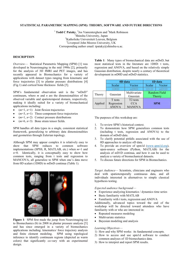
SPM handles all data types in a single, consistent statistical framework, generalizing to arbitrary data dimensionalities and geometries through Eulerian topology. Although SPM may appear complex it is relatively easy to show that SPM reduces to common software implementations (SPSS, R, MATLAB, etc.) when m=1 and n=0. Identically, it is conceptually easy to show how common tests, ranging from t tests and regression to MANCOVA, all generalize to SPM when one’s data move from 0D scalars (1D0D) to mDnD continua (Table 1). Figure 1: SPM first made the jump from Neuroimaging (a) to Biomechanics (b) in 2008 in plantar pressure analysis [5] and has since emerged in a variety of biomechanics applications including: kinematics/ force trajectory analysis and finite element modeling. SPM using topological inference to identify continuum regions (depicted as warm colors) that significantly co-vary with an experimental design. Table 1: Many types of biomechanical data are mDnD, but most statistical tests in the literature are 1D0D: t tests, regression and ANOVA, and based on the relatively simple Gaussian distribution, despite nearly a century of theoretical development in mD0D and mDnD statistics. 0D data 1D data Scalar Vector Scalar Vector 1D0D mD0D 1D1D mD1D Theory Gaussian Multivariate Gaussian Random Field Theory Applied T tests Regression ANOVA T2 tests CCA MANOVA SPM The purposes of this workshop are:

  • 1. To review SPM’s historical context.
  • 2. To demonstrate how SPM generalizes common tests

(including t tests, regression and ANOVA) to the domain of mDnD data.

  • 3. To clarify potential pitfalls associated with the use of

0D approaches to analyze nD data.

  • 4. To provide an overview of spm1d (www.spm1d.org),
  • pen-source software (Python, MATLAB) for the

analysis of mD1D continua, and how it can be used to analyze a variety of biomechanical datasets.

  • 5. To discuss future directions for SPM in Biomechanics.

Target Audience— Scientists, clinicians and engineers who deal with spatiotemporally continuous data, and all individuals interested in alternatives to simple classical hypothesis testing. Expected audience background—

  • Experience analyzing kinematics / dynamics time series
  • Basic familiarity with MATLAB
  • Familiarity with t tests, regression and ANOVA

Additionally, advanced topics toward the end of the workshop will be directed toward attendees who have familiarity with or who are interested in:

  • Repeated measures modeling
  • Multivariate statistics
  • Bayesian modeling and analysis

Learning Objectives— 1) How and why SPM works: its fundamental concepts. 2) How to access and use spm1d software to conduct common analyses of 1D biomechanics data. 3) How to interpret and report SPM results.

slide-2
SLIDE 2

PROGRAM Time Speaker Content 0:00 – 0:30 Pataky Background & Theory 0:30 – 1:00 Robinson Software 1:00 – 1:30 Vanrenterghem Interpretation & Reporting 1:30 – 1:45 Pataky Future Directions 1:45 – 2:00 (None) Open Discussion (The last 5 minutes of each session will be devoted to Q&A) Background & Theory— First we promote critical thinking regarding statistics by interactively reviewing the meaning

  • f experimentation, random sampling and probability
  • values. Through random simulations of 0D data and 1D data

we clarify that statistical tests, while used for experimental analyses, are more aptly summarized as descriptors of

  • randomness. This will prepare attendees to make the

apparent leap but actual small step into the world of SPM: by observing what 1D randomness looks like (Fig.2), and how it can be funneled into t tests, just like the 0D Gaussian, it will become easy for attendees to conceptually connect the simple t test to its nD SPM manifestations (Table 1). Just as t tests’ p values emerge directly from Gaussian theory, SPM’s p values emerge directly from RFT. Coupled with an explanation of SPM’s evolution in both Neuroimaging and Biomechanics, attendees will understand that SPM represents a natural progression of classical statistics concepts. Figure 2: Depiction of Random Field Theory’s model of 1D randomness. Fluctuations about means are modeled as smooth continua, parameterized by the FWHM (full-width at half-maximum) of a Gaussian kernel which is convolved with pure 1D noise. As FWHM approaches ∞, the data approach 0D, and SPM results approach those from common software implementations. By seeing how both 0D Gaussian data and these random can be routed into a t test, attendees will realize that t tests (and all other tests) simply funnel randomness into a test statistic, and thus the only difference between SPM and common 0D techniques is the form of randomness one assumes. Software— Procedural knowledge will be stressed through a Matlab demonstration of spm1d basics (www.spm1d.org), its relation to other software packages, and its broader capabilities. Data

  • rganization

and tests’

  • ptional

parameters (e.g. one- vs. two-tailed, sphericity assumptions, etc.) will be described through example and with reference to online documentation. Additionally, spm1d’s collection

  • f real and simulated datasets will be introduced and
  • explored. We’ll finally introduce spm1d’s online forums for

free software support and general statistics discussion. Interpretation & Reporting— We will next guide attendees through experimental design, scientific interpretation and reporting of SPM results. Necessary details including experimental design parameters, SPM-specific parameters, will be emphasized. Key literature references will be

  • summarized. For a practical demonstration we will revisit

some datasets from our own papers to discuss real Methods and Results reporting. We emphasize these points through hypothetical examples of bad SPM reporting. We finish by summarizing literature and internet resources for continued SPM learning. Future Directions— We will provide an update regarding spm1d’s current state, including a variety of functionality we have in the development pipeline including: normality, power analysis, and Bayesian inference. We will also discuss spm1d’s possible expansion into the 2D and 3D domains, as a light-weight Biomechanics-friendly version of gold-standard Neuroimaging software. We will also briefly revisit theory to summarize SPM’s relation to other whole- dataset techniques from the Biomechanics literature including: principal components analysis, wavelet analysis and functional data analysis. We will end with an open Q&A session regarding our spm1d software, SPM methodology in general, and other aspect of the workshop. LIST OF SPEAKERS (page 3) REFERENCES

  • 1. Friston KJ, et al. Statistical Parametric Mapping: The

Analysis of Functional Brain Images, Elsevier, 2007.

  • 2. Friston KJ, et al. Human Brain Mapping. 2(4), 189-210,

1995.

  • 3. Pataky TC, et al. Journal of Biomechanics 46(14):

2394-2401, 2013.

  • 4. Pataky TC, et al. Journal of Biomechanics, 41(9),

1987-1994, 2008.

  • 5. Li W, et al. Bone, 44(4), 596-602, 2009.
slide-3
SLIDE 3

LIST OF SPEAKERS Todd C. Pataky, Ph.D., Associate Professor Institute for Fiber Engineering, Shinshu University Department of Bioengineering Tokida 3-15-1, Ueda, Nagano, JAPAN 386-8567 tpataky@shinshu-u.ac.jp Todd Pataky received a Ph.D. in Kinesiology and Mechanical Engineering from the Pennsylvania State University in 2004 and pursued postdoctoral research positions in functional neuroimaging and biomechanical continuum analysis in Japan (ATR International, Kyoto) and the UK (University of Liverpool). He is currently an Associate Professor in the Institute for Fiber Engineering, Shinshu University (Japan) where his research focuses on the development of continuum statistics techniques and their applications in Biomechanics. He has over 60 peer-reviewed publications in Biomechanics, many of which focus on SPM and its applications. Notable honors include: Young Investigator Award (bronze) at the World Congress on Biomechanics (2010), Nike Award for Athletic Footwear Research (2009), and William Evans Fellow at the University of Otago, New Zealand (2014). Mark Robinson, Ph.D., Senior Lecturer Research Institute for Sport and Exercise Sciences Liverpool John Moores University Tom Reilly Building, Byrom Street Liverpool, UK L3 3AF M.A.Robinson@ljmu.ac.uk Mark is currently a Senior Lecturer in Biomechanics and Programme Leader for the BSc(Hons) Sport and Exercise Sciences degree at LJMU. He completed his doctorate in 2011 in the School of Sport and Exercise Sciences, LJMU. His research interests are related to musculoskeletal loading, injury and impairment in the lower limbs, specifically during dynamic sporting activities. Of particular interest are knee injuries, player loading in soccer, and gait analysis. His research also includes the development of SPM as a method to provide biomechanists with the appropriate statistical tools to analyze complex biomechanical data. He has published over 30 journal articles in these areas since 2012 and was awarded a UEFA Research Grant in 2014. Jos Vanrenterghem, Ph.D., Associate Professor KU Leuven, Department of Rehabilitation Sciences Tervuursevest 101 - box 1501 3001 Leuven, Belgium jos.vanrenterghem@kuleuven.be Jos received a PhD in Biomechanics from Ghent University in 2004. After having lectured at the School of Sport and Exercise Sciences at Liverpool John Moores University for 10 years, he is now an Associate Professor at the University of Leuven. He has published over 50 articles in peer-reviewed Biomechanics journals, with research interests in lower extremity musculoskeletal loading mechanisms and injury prevention in sport. He has been teaching biomechanics across undergraduate and postgraduate levels, providing him with a good insight in the common issues that students face when analyzing biomechanical data. He has also delivered a series of workshops on research practice in Biomechanics, and devotes much of his work to making biomechanics available in applied and clinical contexts, including through the use of SPM.

slide-4
SLIDE 4

STATISTICAL PARAMETRIC MAPPING

THEORY, SOFTWARE AND FUTURE DIRECTIONS

26 July 2017

ISB Brisbane

Todd Pataky Jos Vanrenterghem Mark Robinson

  • Dept. of Bioengineering
  • Dept. of Rehabilitation

Sciences Institute for Sport and Exercise Sciences

slide-5
SLIDE 5

Overview

  • 17:00 – 17:30

Background & Theory

  • 17:30 – 18:00

Software

  • 18:00 – 18:30

Interpretation & Reporting

  • 18:30 – 18:40

Future Directions

  • 18:40 –

Open Discussion

26 July 2017

ISB Brisbane

slide-6
SLIDE 6

BACKGROUND & THEORY

Todd Pataky

26 July 2017

ISB Brisbane

slide-7
SLIDE 7

S P M

STATISTICAL Probabilistic inferences regarding experimental data PARAMETRIC

  • Based on mean & SD & sample size
  • Also non-parametric (SnPM)
  • Parameterized model of cerebral blood flow

MAPPING Results form an n-Dimensional “map” in the same space as the original data (i.e. test statistics [t and F] are n-D continua)

slide-8
SLIDE 8

n-D continua Smooth, bounded

slide-9
SLIDE 9

Univariate 0D

Body mass 0D, 1D

Multivariate 0D

GRF at t = 50 ms 0D, 3D

Univariate nD

Foot pressure 2D, 1D

Multivariate nD

Bone strain tensor 3D, 6D

Univariate 1D

Knee flexion 1D, 1D

Multivariate 1D

Knee posture 1D, 6D

n-D, m-D continua

continuum dependent variable

SPSS MATLAB R

slide-10
SLIDE 10

A brief history of SPM

1976 Adler & Hasofer, Annals of Prob. 1990 Friston et al. J Cerebral Blood Flow 1995 Friston et al. Human Brain Mapping 2004 Worsley et al. NeuroImage 2008 Pataky et al. New insights into the plantar pressure correlates

  • f walking speed using pedobarographic statistical parametric mapping

J Biomech 41: 1987-1994. 8663 citations H-index: 202

2009 Li et al. Identify fracture-critical regions inside the proximal

femur using statistical parametric mapping, Bone 44: 596-602 i-10-index: 758

slide-11
SLIDE 11
slide-12
SLIDE 12

Example

slide-13
SLIDE 13

What is a p value?

Demo

slide-14
SLIDE 14

What is a p value?

The probability that a random process will yield a particular result.

slide-15
SLIDE 15

Random data Experiment p value Metric

t value two sample

Infinite set of experiments One experiment

slide-16
SLIDE 16

t and F values describe one experiment p values describe the behavior of random data in an infinite set of experiments

Use nD random data to make probabilistic conclusions regarding nD experimental data

slide-17
SLIDE 17

www.spm1d.org

slide-18
SLIDE 18
slide-19
SLIDE 19

spm1d.org/rft1d

Pataky (2016) J. Statistical Software

slide-20
SLIDE 20
slide-21
SLIDE 21

Statistics

  • z
  • t
  • F
  • 𝛙2
  • T2

Distribution Functions

  • probability density
  • survival function
  • inverse survival function
slide-22
SLIDE 22

Science

Classical hypothesis testing

MANCOVA

Bayesian

Engineering

Dimensionality reduction

PCA ICA kPCA

Machine learning

ANN SVM SOM

slide-23
SLIDE 23

www.spm1d.org

slide-24
SLIDE 24

spm1d tutorial, ISB 2017

Mark A. Robinson Liverpool John Moores University, UK m.a.robinson@ljmu.ac.uk This tutorial will focus on using the software and will cover:

  • 1. getting "spm1d"
  • 2. input data organisation
  • 3. statistical tests: t-tests, regression, ANOVA, CCA
  • 4. keywords
  • 5. help
  • 6. questions?
  • 1. Software

"spm1d" is an open source package for one-dimensional Statistical Parametric Mapping. The current version is 0.4 The python code repository is: https://github.com/0todd0000/spm1d/ (https://github.com/0todd0000/spm1d/) The matlab code repository is: https://github.com/0todd0000/spm1dmatlab (https://github.com/0todd0000/spm1dmatlab)

  • 2. Input data organisation
slide-25
SLIDE 25
  • 2. Input data organisation

Univariate spm1d uses a (J x Q) array, where J is the number of 1D responses (i.e. trials or subjects) and Q is the number of nodes in the 1D continuum. e.g. 10 subject means normalized to 101 nodes will give a 10x101 array Multivariate spm1d analysis the data should be arranged as a (J x Q x I) array, where I is the number of vector components in the 1D continuum. e.g. 10 subject means normalized to 101 nodes for GRF X,Y,Z, will give a 10x101x3 vector field

  • 3. Statistical tests
  • a. 1D two-sample t-test

/examples/stats1d/ex1d_ttest2.m

slide-26
SLIDE 26

In [2]: % load some data dataset = spm1d.data.uv1d.t2.PlantarArchAngle(); [YA,YB] = deal(dataset.YA, dataset.YB); dataset

This dataset has two variables both of size 10x101 spm1d has built in plotting functions for data e.g. plot_meanSD

dataset = struct with fields: cite: 'Caravaggi, P., Pataky, T., G?nther, M., S avage, R., & Crompton, R. (2010). Dynamics of longit udinal arch support in relation to walking speed: co ntribution of the plantar aponeurosis. Journal of An atomy, 217(3), 254?261. http://doi.org/10.1111/j.146 9-7580.2010.01261.x' YA: [10×101 double] YB: [10×101 double]

slide-27
SLIDE 27

In [3]: % Plot the data spm1d.plot.plot_meanSD(YA,'color','r'); hold on spm1d.plot.plot_meanSD(YB,'color','b');

slide-28
SLIDE 28

In [4]: %(1) Conduct SPM analysis: spm = spm1d.stats.ttest2(YA, YB); spmi = spm.inference(0.05, 'two_tailed',true); disp(spmi) SPM{t} inference z: [1×101 double] df: [1 18] fwhm: 20.5956 resels: [1 4.8554] alpha: 0.0500 zstar: 3.2947 p_set: 0.0312 p: 0.0312

slide-29
SLIDE 29

In [5]: % Plot SPM analysis outcome spmi.plot(); spmi.plot_threshold_label(); spmi.plot_p_values();

slide-30
SLIDE 30

In [6]: % For descriptive information about clusters spmi.clusters{1,1}

  • b. 1D Linear Regression

/examples/stats1d/ex1d_regression.m

ans = Cluster with properties: endpoints: [93.2746 100] csign: 1 iswrapped: 0 extent: 6.7254 extentR: 0.3265 h: 3.2947 xy: [96.5343 4.5976] P: 0.0312

slide-31
SLIDE 31

In [7]: % Load example data dataset = spm1d.data.uv1d.regress.SpeedGRF(); [Y,x] = deal(dataset.Y, dataset.x); dataset dataset = struct with fields: cite: 'Pataky, T. C., Caravaggi, P., Savage, R., Parker, D., Goulermas, J., Sellers, W., & Crompton,

  • R. (2008). New insights into the plantar pressure co

rrelates of walking speed using pedobarographic stat istical parametric mapping (pSPM). Journal of Biomec hanics, 41(9), 1987?1994.' Y: [60×101 double] x: [60×1 double]

slide-32
SLIDE 32

In [8]: % Plot the GRF data plot(Y'); xlabel('Stance %'); ylabel('Force (N/BW)');

slide-33
SLIDE 33

In [9]: subplot(221); scatter(x,Y(:,20)); title('20%'); xlabel('speed (m/s)'); yla bel('Force (N/BW)'); lsline() subplot(222); scatter(x,Y(:,50)); title('50%'); xlabel('speed (m/s)'); yla bel('Force (N/BW)'); lsline() subplot(223); scatter(x,Y(:,92)); title('92%'); xlabel('speed (m/s)'); yla bel('Force (N/BW)'); lsline()

slide-34
SLIDE 34

In [10]: % Conduct SPM analysis: spm = spm1d.stats.regress(Y, x); spmi = spm.inference(0.05, 'two_tailed', true); disp(spmi) SPM{t} inference z: [1×101 double] df: [1 58] fwhm: 6.1343 resels: [1 16.3017] alpha: 0.0500 zstar: 3.3945 p_set: 4.0634e-14 p: [0 0 0 0.0017]

slide-35
SLIDE 35

In [11]: % Plot SPM output spmi.plot(); spmi.plot_threshold_label(); spmi.plot_p_values();

  • c. ANOVA - between groups

/examples/stats1d/ex1d_anova1.m

In [12]: % Load data: dataset = spm1d.data.uv1d.anova1.SpeedGRFcategorical(); [Y,A] = deal(dataset.Y, dataset.A);

slide-36
SLIDE 36

disp('Data Loaded') dataset A Data Loaded dataset = struct with fields: cite: 'Pataky, T. C., Caravaggi, P., Savage, R., Parker, D., Goulermas, J., Sellers, W., & Crompton,

  • R. (2008). New insights into the plantar pressure co

rrelates of walking speed using pedobarographic stat istical parametric mapping (pSPM). Journal of Biomec hanics, 41(9), 1987?1994.' Y: [60×101 double] A: [60×1 uint8] A = 60×1 uint8 column vector 3 1 1 1 3 1 1 2 2 2 3 3

slide-37
SLIDE 37

2 1 3 1 3 1 3 2 1 1 3 3 3 2 3 2 2 2 2 3 1 3 3 2 2 1 2 2 2 1 2 2 1 3 3 1

slide-38
SLIDE 38

In [13]: % Run SPM analysis spm = spm1d.stats.anova1(Y, A); spmi = spm.inference(0.05); disp(spmi) 1 2 2 1 1 3 2 1 1 3 3 3 SPM{F} inference z: [1×101 double] df: [2 57] fwhm: 6.1179 resels: [1 16.3455] alpha: 0.0500 zstar: 7.5969 p_set: 5.2921e-12 p: [2.2204e-16 3.2533e-06]

slide-39
SLIDE 39

In [14]: % Plot spmi.plot(); spmi.plot_threshold_label(); spmi.plot_p_values();

slide-40
SLIDE 40

In [15]: % Post-hoc Analysis % separate into groups: Y1 = Y(A==1,:); Y2 = Y(A==2,:); Y3 = Y(A==3,:); % Conduct post-hoc analysis: t21 = spm1d.stats.ttest2(Y2, Y1); t32 = spm1d.stats.ttest2(Y3, Y2); t31 = spm1d.stats.ttest2(Y3, Y1); % inference: alpha = 0.05; nTests = 3; p_critical = spm1d.util.p_critical_bonf(alpha, nTests); t21i = t21.inference(p_critical, 'two_tailed',true); t32i = t32.inference(p_critical, 'two_tailed',true); t31i = t31.inference(p_critical, 'two_tailed',true);

slide-41
SLIDE 41

In [16]: subplot(221); t21i.plot(); title('t21') subplot(222); t32i.plot(); title('t32') subplot(223); t31i.plot(); title('t31')

  • d. Canonical Correlation Analysis

/examples/stats1d/ex1d_cca.m

slide-42
SLIDE 42

In [17]: %(0) Load data: dataset = spm1d.data.mv1d.cca.Dorn2012(); [Y,x] = deal(dataset.Y, dataset.x); dataset x In [18]: dataset = struct with fields: cite: 'Dorn, T. W., Schache, A. G., & Pandy, M.

  • G. (2012). Muscular strategy shift in human running:

dependence of running speed on hip and ankle muscle

  • performance. Journal of Experimental Biology, 215(11

), 1944?1956. http://doi.org/10.1242/jeb.064527' www: 'https://simtk.org/home/runningspeeds' Y: [8×100×3 double] x: [8×1 double] x = 3.5600 3.5600 5.2000 5.2000 7.0000 7.0000 9.4900 9.4900

slide-43
SLIDE 43

In [18]: % Visualise this dataset plot(Y(:,:,1)','r'); hold on plot(Y(:,:,2)','g'); plot(Y(:,:,3)','b'); x x = 3.5600 3.5600 5.2000 5.2000 7.0000 7.0000 9.4900 9.4900

slide-44
SLIDE 44

In [19]: %(1) Conduct SPM analysis: spm = spm1d.stats.cca(Y, x); spmi = spm.inference(0.05); disp(spmi) SPM{X2} inference z: [1×100 double] df: [1 3] fwhm: 8.8974 resels: [1 11.1269] alpha: 0.0500 zstar: 14.9752 p_set: 5.6243e-10 p: [3.3539e-05 1.2275e-06]

slide-45
SLIDE 45

In [20]: %(2) Plot spmi.plot(); spmi.plot_threshold_label(); spmi.plot_p_values();

  • 4. Keywords

Equality of variance t = spm1d.stats.ttest2(YA, YB, 'equal_var', false) One or two-tailed Interpolation of clusters

slide-46
SLIDE 46

ti = t.inference(0.05, 'two_tailed', false, 'interp', true) Circular fields ti = t.inference(0.05, 'circular', true)

Region of interest

slide-47
SLIDE 47

In [21]: dataset = spm1d.data.uv1d.t1.SimulatedPataky2015a(); [Y,mu] = deal(dataset.Y, dataset.mu); % Create a region of interest (ROI): roi = false( 1, size(Y,2) ); roi(71:80) = true; plot(roi); title('Defined ROI');

slide-48
SLIDE 48

In [22]: %(1) Conduct SPM analysis: spm = spm1d.stats.ttest(Y - mu, 'roi', roi); spmi = spm.inference(0.05, 'two_tailed', false, 'interp',true) ; plot(spmi)

  • 5. Help

spm1d website: www.spm1d.org matlab help forum: https://github.com/0todd0000/spm1dmatlab/issues (https://github.com/0todd0000/spm1dmatlab/issues) Python help forum: https://github.com/0todd0000/spm1d/issues (https://github.com/0todd0000/spm1d/issues)

slide-49
SLIDE 49

INTERPRETATION & REPORTING

Jos Vanrenterghem

26 July 2017

ISB Brisbane

slide-50
SLIDE 50

Reporting SPM methods

26 July 2017

ISB Brisbane

slide-51
SLIDE 51

SPM Methods

[Data treatment – smoothing, averaging] a) Statistical tests used b) SPM code & analysis software c) Refer to key SPM/RFT literature

– Friston KJ, Holmes AP, Worsley KJ, Poline JB, Frith CD, Frackowiak RSJ (1995). Statistical parametric maps in functional imaging: a general linear approach. Human Brain Mapping 2, 189–210. – SPM documentation repository, Wellcome Trust Centre for Neuroimaging: http://www.fil.ion.ucl.ac.uk/spm/doc/

26 July 2017

ISB Brisbane

slide-52
SLIDE 52

SPM Methods

[Data treatment – smoothing, averaging] a) Statistical tests used b) SPM code & analysis software c) Refer to key SPM/RFT literature d) Define terminology e) Specify alpha – correction? f) How results will be interpreted

26 July 2017

ISB Brisbane

slide-53
SLIDE 53

Example

Statistical parametric mapping (SPM, Friston et al., 2007) was used to statistically compare walking speeds. Specifically a SPM two-tailed paired t-test was used to compare the longitudinal arch angle during normal versus fast walking (α=0.05). The scalar output statistic, SPM{t}, was calculated separately at each individual time node and is referred to as a Statistical Parametric Map. At this stage it is worth noting that SPM refers to the overall methodological approach, and SPM{t} to the scalar trajectory variable. The calculation of SPM{t} simply indicates the magnitude of the Normal-Fast differences, therefore with this variable alone we cannot accept or reject our null hypothesis. To test our null hypothesis we next calculated the critical threshold at which only α % (5%) of smooth random curves would be expected to traverse. This threshold is based upon estimates of trajectory smoothness via temporal gradients [Friston et al., 2007] and, based on that smoothness, Random Field Theory expectations regarding the field-wide maximum [Adler and Taylor, 2007]. Conceptually, a SPM paired t-test is similar to the calculation and interpretation of a scalar paired t- test; if the SPM{t} trajectory crosses the critical threshold at any time node, the null hypothesis is rejected. Typically, due to waveform smoothness and the inter-dependence of neighbouring points, multiple adjacent points of the SPM{t} curve often exceed the critical threshold, we therefore call these “supra-threshold clusters”. SPM then uses Random Field Theory expectations regarding supra-threshold cluster size to calculate cluster specific p-values which indicate the probability with which supra-threshold clusters could have been produced by a random field process with the same temporal smoothness [Adler and Taylor, 2007]. All SPM analyses were implemented using the open-source spm1d code (v.M0.1, www.spm1d.org) in Matlab (R2014a, 8.3.0.532, The Mathworks Inc, Natick, MA). 26 July 2017

ISB Brisbane

slide-54
SLIDE 54

Example

Statistical parametric mapping (SPM, Friston et al., 2007) was used to statistically compare walking speeds. Specifically a SPM two-tailed paired t-test was used to compare the longitudinal arch angle during normal versus fast walking (α=0.05). The scalar output statistic, SPM{t}, was calculated separately at each individual time node and is referred to as a Statistical Parametric Map. At this stage it is worth noting that SPM refers to the overall methodological approach, and SPM{t} to the scalar trajectory variable. The calculation of SPM{t} simply indicates the magnitude of the Normal-Fast differences, therefore with this variable alone we cannot accept or reject our null hypothesis. To test our null hypothesis we next calculated the critical threshold at which only α % (5%) of smooth random curves would be expected to traverse. This threshold is based upon estimates of trajectory smoothness via temporal gradients [Friston et al., 2007] and, based on that smoothness, Random Field Theory expectations regarding the field-wide maximum [Adler and Taylor, 2007]. Conceptually, a SPM paired t-test is similar to the calculation and interpretation of a scalar paired t- test; if the SPM{t} trajectory crosses the critical threshold at any time node, the null hypothesis is rejected. Typically, due to waveform smoothness and the inter-dependence of neighbouring points, multiple adjacent points of the SPM{t} curve often exceed the critical threshold, we therefore call these “supra-threshold clusters”. SPM then uses Random Field Theory expectations regarding supra-threshold cluster size to calculate cluster specific p-values which indicate the probability with which supra-threshold clusters could have been produced by a random field process with the same temporal smoothness [Adler and Taylor, 2007]. All SPM analyses were implemented using the open-source spm1d code (v.M0.1, www.spm1d.org) in Matlab (R2014a, 8.3.0.532, The Mathworks Inc, Natick, MA). 26 July 2017

ISB Brisbane

slide-55
SLIDE 55

26 July 2017

ISB Brisbane

To compare between groups, a curve analysis was performed using statistical parametric mapping (SPM) (13). Initially, ANOVA over the normalized time series was used to establish the presence of any significant differences between the three groups. If statistical significance was reached, post hoc t-tests over the normalized time series were used to determine between which groups significant differences occurred. For both the ANOVA and t-test analyses, SPM involved four steps. The first was computing the value of a test statistic at each point in the normalized time

  • series. The second was estimating temporal smoothness on the

basis of the average temporal gradient. The third was computing the value of test statistic above which only > = 5% of the data would be expected to reach had the test statistic trajectory resulted from an equally smooth random process. The last was computing the probability that specific suprathreshold regions could have resulted from an equivalently smooth random process. Technical details are provided elsewhere (13,27).

slide-56
SLIDE 56

Reporting SPM results t-tests

26 July 2017

ISB Brisbane

slide-57
SLIDE 57

26 July 2017

ISB Brisbane

slide-58
SLIDE 58

the “SPM” variable

26 July 2017

ISB Brisbane

slide-59
SLIDE 59

the “SPMi” variable

26 July 2017

ISB Brisbane

slide-60
SLIDE 60

Random data Experiment p value Metric

t value two sample

Infinite set of experiments One experiment

slide-61
SLIDE 61

SPM and SPMi

SPM

Name Size or value STAT T z 1x100 double nNodes 100

df

[1,9] fwhm 11.2192 resels [1,8.8242] sigma2 1x100 double r [] isregress beta 1x100 double R 10x100 double

SPMi

Name Size or value alpha 0.05 two_tailed zstar 3.8213 h0reject 1 p_set 0.031 p 0.031 nClusters 1 clusters 1x1 cell

26 July 2017

ISB Brisbane

slide-62
SLIDE 62

Results

Key information to present: a) Was the critical threshold exceeded? b) Direction of effect c) Consequence for the null hypothesis d) Descriptive data:

critical threshold, p-value/s, number of supra-threshold clusters, extent of clusters, degrees of freedom.

26 July 2017

ISB Brisbane

slide-63
SLIDE 63

Results section bad example

The mean arch angles during normal and fast walking were highly similar for the majority of time except for the very last bit of the walking cycle (figure 1a). The arch angle during fast walking were significantly different between normal and fast walking (figure 1b, p=0.024).

26 July 2017

ISB Brisbane

slide-64
SLIDE 64

Results section ‘better’ example

The mean arch angles during normal and fast walking were highly similar for the majority of time (figure 1a). However one supra-threshold cluster (96-100%) exceeded the critical threshold of 3.933 as the arch angle during fast walking was significantly more negative than during normal walking (figure 1b). The precise probability that a supra-threshold cluster of this size would be observed in repeated random samplings was p=0.024. The null hypothesis was therefore rejected.

26 July 2017

ISB Brisbane

slide-65
SLIDE 65

Figure caption

Figure 1 a) Mean trajectories for longitudinal arch angles during normal (black) and fast (red) walking. b) The paired samples t- test statistic SPM {t}. The critical threshold of 3.933 (red dashed line) was exceeded at time = 96% with a supra-threshold cluster probability value of p=0.024 indicating a significantly more negative angle in the fast condition.

26 July 2017

ISB Brisbane

slide-66
SLIDE 66

Reporting SPM results Regression

26 July 2017

ISB Brisbane

slide-67
SLIDE 67

Regression

spm = spm1d.stats.regress(Y, x); spmi = spm.inference(0.05, 'two_tailed', true);

“x” independent variable

walking speed

“Y” dependent variable vertical GRF trajectories

26 July 2017

ISB Brisbane

slide-68
SLIDE 68

SPM output

26 July 2017

ISB Brisbane

slide-69
SLIDE 69

SPM output

26 July 2017

ISB Brisbane

The t value is the statistic upon which statistical inferences (p values) are based. The regression coefficient r and t value are alternative expressions of effect magnitude, and map directly to each other given the sample size.

slide-70
SLIDE 70

Regression interpretation

There was a significant relationship between walking speed and vGRF. A greater walking speed significantly increased the vGRF during the first and last 30% stance but significantly reduced GRF from ~30-70% stance. As random data would produce this effect <5% time the null hypothesis was therefore rejected.

26 July 2017

ISB Brisbane

slide-71
SLIDE 71

Example methods/results

  • Pataky TC (2010). Generalized n-dimensional biomechanical field analysis using statistical

parametric mapping. Journal of Biomechanics 43, 1976-1982.

  • Pataky TC (2012) One-dimensional statistical parametric mapping in Python. Computer

Methods in Biomechanics and Biomedical Engineering. 15, 295-301.

  • Pataky TC, Robinson MA, Vanrenterghem J (2013). Vector field statistical analysis of kinematic

and force trajectories. Journal of Biomechanics 46 (14): 2394-2401.

Applications

  • Vanrenterghem, J., Venables, E., Pataky, T., Robinson, M. (2012). The effect of running speed
  • n knee mechanical loading in females during side cutting. Journal of Biomechanics, 45,

2444-2449.

  • De Ridder, R., Willems, T., Vanrenterghem, J., Robinson, M., Pataky, T., Roosen, P. (2013). Gait

kinematics of subjects with chronic ankle instability using a multi-segmented foot model. Medicine and Science in Sports and Exercise, 45, 2129-2136.

  • Robinson, M.A., Donnelly, C.J., Tsao, J., Vanrenterghem, J. (2014). Impact of knee modelling

approach on indicators and classification of ACL injury risk. Medicine & Science in Sports & Exercise, 46 (7), 1269-1276.

www.spm1d.org

26 July 2017

ISB Brisbane