Statistical Learning: The Complex Cases Case 0: Bayesian Network - PDF document

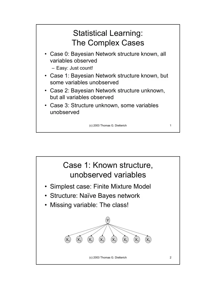
Statistical Learning: The Complex Cases • Case 0: Bayesian Network structure known, all variables observed – Easy: Just count! • Case 1: Bayesian Network structure known, but some variables unobserved • Case 2: Bayesian Network structure unknown, but all variables observed • Case 3: Structure unknown, some variables unobserved (c) 2003 Thomas G. Dietterich 1 Case 1: Known structure, unobserved variables • Simplest case: Finite Mixture Model • Structure: Naïve Bayes network • Missing variable: The class! Y X 1 X 1 X 1 X 1 X 1 X 1 X 1 X 1 (c) 2003 Thomas G. Dietterich 2 1

Example Problem: Cluster Wafers for HP • We wish to learn C P(C,X 1 ,X 2 , …, X 105 ) • C is a hidden “class” X1 X2 X3 X4 X5 X6 X105 variable (c) 2003 Thomas G. Dietterich 3 Complete Data and Incomplete data Wafer X 1 X 2 … X 105 C 1 1 1 … 0 ? 2 0 1 … 1 ? 3 0 1 … 1 ? 4 1 0 … 1 ? • The given data are incomplete. If we could guess the values of C, we would have complete data, and learning would be easy (c) 2003 Thomas G. Dietterich 4 2

“Hard” EM • Let W = (X 1 , X 2 , …, X 105 ) be the observed wafers • Guess initial values for C (e.g., randomly) • Repeat until convergence – Hard M-Step: (Compute maximum likelihood estimates from complete data) • Learn P(C) • Learn P(X i |C) for all I – Hard E-Step: (Re-estimate the C values) • For each wafer, set C to maximize P(W|C) (c) 2003 Thomas G. Dietterich 5 Hard EM Example • Suppose we have 10 chips per wafer and 2 wafer classes. Suppose this is the “true” distribution: P(X i =1|C) 0 1 X 1 0.34 0.41 C P(C) X 2 0.19 0.83 0 0.58 X 3 0.20 0.15 X 4 0.69 0.19 1 0.42 X 5 0.57 0.53 X 6 0.71 0.93 Draw 100 training examples X 7 0.34 0.68 and 100 test examples from X 8 0.43 0.04 this distribution X 9 0.13 0.65 X 10 0.14 0.89 (c) 2003 Thomas G. Dietterich 6 3

Fit of Model to Fully-Observed Training Data P(X i =1|C) 0 1 X 1 0.28 0.41 C P(C) X 2 0.15 0.85 0 0.61 X 3 0.15 0.13 1 0.39 X 4 0.67 0.23 X 5 0.49 0.51 X 6 0.74 0.97 X 7 0.39 0.69 X 8 0.34 0.03 X 9 0.10 0.67 X 10 0.16 0.87 • Hard-EM could achieve this if it could correctly guess C for each example (c) 2003 Thomas G. Dietterich 7 EM Training and Testing Curve -790 Training Set -800 -810 -820 Testing Set Log likelihood -830 -840 -850 -860 -870 -880 0 2 4 6 8 10 Iteration (c) 2003 Thomas G. Dietterich 8 4

Hard EM Fitted Model P(X i =1|C) 0 1 X 1 0.35 0.32 C P(C) X 2 0.81 0.12 0 0.43 X 3 0.09 0.18 1 0.57 X 4 0.26 0.68 X 5 0.60 0.42 X 6 0.95 0.74 • Note that the classes are X 7 0.65 0.40 “reversed”: The learned X 8 0.02 0.37 class 0 corresponds to X 9 0.67 0.05 the true class 1. But the X 10 0.86 0.12 likelihoods are the same if the classes are reversed (c) 2003 Thomas G. Dietterich 9 The search can get stuck in local minima P(X i =1|C) 0 1 X 1 0.35 0.00 C P(C) X 2 0.42 0.43 0 0.93 X 3 0.12 0.43 1 0.07 X 4 0.47 0.86 X 5 0.53 0.14 X 6 0.83 0.86 X 7 0.51 0.57 • Parameters can go to X 8 0.16 1.00 zero or one! X 9 0.34 0.00 X 10 0.47 0.00 • Should use Laplace Estimates (c) 2003 Thomas G. Dietterich 10 5

The Expectation-Maximization (EM) Algorithm • Initialize the probability tables randomly • Repeat until convergence – E-Step: For each wafer, compute P’(C|W) – M-Step: Compute maximum likelihood estimates from weighted data (S) We treat P’(C|W) as fractional “counts”. Each wafer W i belongs to class C with probability P’(C|W). (c) 2003 Thomas G. Dietterich 11 EM Training Curve -780 -790 Training -800 -810 log likelihood -820 -830 Testing -840 -850 -860 -870 0 10 20 30 40 50 60 Iteration • Each iteration is guaranteed to increase the likelihood of the data. Hence, EM is guaranteed to converge to a local maximum of the likelihood. (c) 2003 Thomas G. Dietterich 12 6

EM Fitted Model P(X i =1|C) 0 1 C P(C) X 1 0.41 0.28 0 0.35 X 2 0.81 0.21 X 3 0.11 0.15 1 0.65 X 4 0.26 0.63 X 5 0.56 0.47 X 6 0.97 0.75 X 7 0.74 0.38 X 8 0.00 0.34 X 9 0.76 0.08 X 10 0.96 0.16 (c) 2003 Thomas G. Dietterich 13 Avoiding Overfitting • Early stopping. Hold out some of the data, monitor log likelihood on this holdout data, and stop when it starts to decrease • Laplace estimates • Full Bayes (c) 2003 Thomas G. Dietterich 14 7

EM with Laplace Corrections -790 Training -800 -810 -820 log likelihood Testing -830 -840 Dirichlet = 0 -850 -860 -870 -880 0 10 20 30 40 50 60 EM iterations • When correction is removed, EM overfits immediately (c) 2003 Thomas G. Dietterich 15 Comparison of Results Method Training Set Test Set true model -802.85 -816.40 hard-EM -791.69 -826.94 soft-EM -790.97 -827.27 soft-EM + -794.31 -823.19 Laplace (c) 2003 Thomas G. Dietterich 16 8

Graphical Comparison -770.00 true model hard-EM soft-EM soft-EM + Laplace -780.00 -790.00 Training Set -800.00 Test Set -810.00 -820.00 -830.00 • hard-EM and soft-EM overfit • soft-EM + Laplace gives best test set result (c) 2003 Thomas G. Dietterich 17 Unsupervised Learning of an HMM • Suppose we are given only the Umbrella observations as our training data • How can we learn P(R t |R t-1 ) and P(U t |R t )? (c) 2003 Thomas G. Dietterich 18 9

EM for HMMs: “The Forward-Backward Algorithm” • Initialize probabilities randomly • Repeat to convergence – E-step: Run the forward-backward algorithm on each training example to compute P’(R t |U 1:N ) for each time step t. – M-step: Re-estimate P(R t |R t-1 ) and P(U t |R t ) treating the P’(R t |U 1:N ) as fractional counts • Also known as the Baum-Welch algorithm (c) 2003 Thomas G. Dietterich 19 Hard-EM for HMMs: Viterbi Training • EM requires forward and backward passes. In the early iterations, just finding the single best path usually works well • Initialize probabilities randomly • Repeat to convergence – E-step: Run the Viterbi algorithm on each training example to compute R’ t = argmax Rt P(R t |U 1:N ) for each time step t. – M-step: Re-estimate P(R t |R t-1 ) and P(U t |R t ) treating the R‘ t as if they were correct labels (c) 2003 Thomas G. Dietterich 20 10

Case 2: All variables observed; Structure unknown • Search the space of structures – For each potential structure • Apply standard maximum likelihood method to fit the parameters • Problem: How to score the structures? – The complete graph will always give the best likelihood on the training data (because it can memorize the data) (c) 2003 Thomas G. Dietterich 21 MAP Approach: M = model; D = data argmax M P(M | D) = argmax M P(D | M) · P(M) argmax M log P(M | D) = argmin M – log P(D | M) – log P(M) –log P(M) = number of bits required to represent M (for some chosen representation scheme) Therefore: – Choose a representation scheme – Measure description length in this scheme – Use this for – log P(M) (c) 2003 Thomas G. Dietterich 22 11

Representation Scheme • Representational cost of adding a parent p to a child node c that already has k parents – Must specify link: log 2 n(n-1)/2 bits – c already requires 2 k parameters. Adding another (boolean) parent will make this 2 k+1 parameters, so the increase is 2 k+1 – 2 k = 2 k each of which requires, say, 8 bits. This gives 8 · 2 k bits – Total: 8 · 2 k + log 2 n(n-1)/2 • Min: – log P(D | M) + λ [ 8 · 2 k + log 2 n(n-1)/2] – λ is adjusted (e.g., by internal holdout data) to give best results (c) 2003 Thomas G. Dietterich 23 Note: There are many other possible representation schemes • Example: Use joint distribution plus the graph structure – Joint distribution always has 2 N parameters – Describe graph by which edges are missing ! – This scheme would assign the smallest description length to the complete graph! • The chosen representation scheme implies a prior belief that graphs that can be described compactly under the scheme have higher prior probability P(M) (c) 2003 Thomas G. Dietterich 24 12

Search Algorithm • Search space is all DAGs with N nodes – Very large! • Greedy method – Operators: Add an edge, Delete an edge, Reverse an edge – At each step, • Apply each operator to change the structure • Fit the resulting graph to the data • Measure total description length • Take the best move – Stop when local maximum is reached (c) 2003 Thomas G. Dietterich 25 Alternative Search Algorithm • Operator: – Delete a node and all of its edges from the graph – Compute the optimal set of edges for the node and re-insert it into the graph • Surprisingly, this can be done efficiently! • Apply this operator greedily (c) 2003 Thomas G. Dietterich 26 13

Initializing the Search • Compute the best tree-structured graph using Chou-Liu Algorithm (c) 2003 Thomas G. Dietterich 27 Chou-Liu Algorithm • for all pairs (X i ,X j ) of variables do – compute mutual information: X P ( x i , x j ) I ( X i ; X j ) = P ( x i , x j ) log P ( x i ) P ( x j ) x i ,x j • Construct complete graph G such that the edge (X i ,X j ) has weight I(X i ;X j ) • Compute maximum weight spanning tree • Choose root node arbitrarily and direct edges away from it recursively (c) 2003 Thomas G. Dietterich 28 14