
SLIDE 1
1
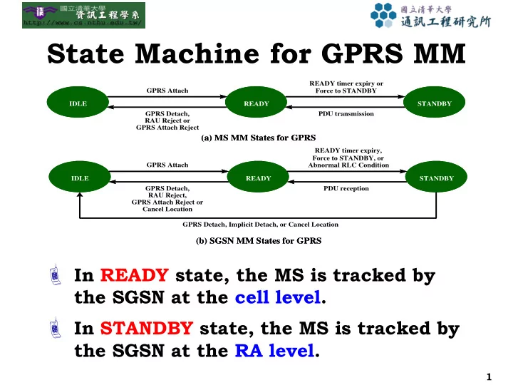
State Machine for GPRS MM
In READY state, the MS is tracked by
the SGSN at the cell level.
In STANDBY state, the MS is tracked by
the SGSN at the RA level.
IDLE READY STANDBY GPRS Attach READY timer expiry or Force to STANDBY PDU transmission IDLE READY STANDBY GPRS Attach GPRS Attach Reject or Cancel Location READY timer expiry, Force to STANDBY, or Abnormal RLC Condition PDU reception GPRS Detach, Implicit Detach, or Cancel Location IDLE READY STANDBY IDLE READY STANDBY GPRS Detach, RAU Reject, GPRS Detach, RAU Reject or GPRS Attach Reject
(b) SGSN MM States for GPRS (b) SGSN MM States for GPRS (a) MS MM States for GPRS (a) MS MM States for GPRS