SLIDE 1
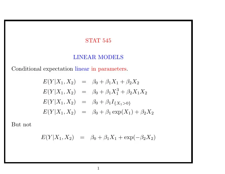
STAT 545 LINEAR MODELS Conditional expectation linear in parameters. E(Y |X1, X2) = β0 + β1X1 + β2X2 E(Y |X1, X2) = β0 + β1X3
1 + β2X1X2
E(Y |X1, X2) = β0 + β1I{X1>0} E(Y |X1, X2) = β0 + β1 exp(X1) + β2X2 But not E(Y |X1, X2) = β0 + β1X1 + exp(−β2X2)
1
SLIDE 2 Notation Repeated realizations of (Y, X1, . . . , Xp), where Y |X1, . . . , Xp ∼ N
- β0 + β1X1 + . . . + βpXp, σ2
Or i = 1, . . . , n indexes observations, j = 1, . . . , p indexes predictors, observe vector of responses Y (entries Yi) and design matrix X (entries Xij). Y |X ∼ Nn(Xβ, σ2In). ML/LS estimator: ˆ β = argminβY − Xβ2 = (XTX)−1XT Y .
2
SLIDE 3
NOTE UBIQUITY OF DESIGN MATRIX, RESPONSE VECTOR FORMULATION: linear regression, multiple linear regression, ANOVA, curve-fitting,.... Software: lm() function. > tmp <- lm(y~x) > coef(tmp) ### or tmp$coef > resid(tmp) ### or tmp$resid > fitted(tmp) ### or tmp$fitted
3
SLIDE 4
Simple Example > attach(whiteside) > plot(Temp, Gas, pch=as.numeric(Insul), col=1+as.numeric(Insul)) > tmp1 <- lm(Gas~Temp, data=whiteside, subset=Insul=="Before") > abline(tmp1, col=2) ... > names(tmp1) [1] "coefficients" "residuals" "effects" [4] "rank" "fitted.values" "assign" [7] "qr" "df.residual" "xlevels" [10] "call" "terms" "model"
4
SLIDE 5 2 4 6 8 10 2 3 4 5 6 7 Temp Gas
5
SLIDE 6 > summary(tmp1) Call: lm(formula = Gas ~ Temp, data = whiteside, subset = ... Residuals: Min 1Q Median 3Q Max
0.06068 0.16770 0.59778 Coefficients: Estimate Std. Error t value Pr(>|t|) (Intercept) 6.85383 0.11842 57.88 <2e-16 *** Temp
0.01959
<2e-16 ***
0 ‘***’ 0.001 ‘**’ 0.01 ‘*’ 0.05 ... Residual standard error: 0.2813 on 24 degrees of freedom Multiple R-Squared: 0.9438, Adjusted R-squared: 0.9415 F-statistic: 403.1 on 1 and 24 DF, p-value: < 2.2e-16
6
SLIDE 7
Model Formulae fake.data <- cbind( data.frame("y"=rnorm(54)), data.frame("x1"=rnorm(54)), data.frame("x2"=rnorm(54)), data.frame("a"=factor(c(rep("ubc",18),rep("sfu",18), rep("vic",18)), levels=c("ubc","sfu","vic"))), data.frame("b"=ordered(rep(c(rep("sm",3),rep("md",3), rep("lg",3)),6), levels=c("sm","md","lg"))), data.frame("c"=factor(rep(c("rd","gr","bl"),18), levels=c("rd","gr","bl"))) )
7
SLIDE 8 > print(fake.data) y x1 x2 a b c 1
1.486 ubc sm rd 2
0.905 ubc sm gr 3 0.179 -1.482 -1.450 ubc sm bl 4
- 0.863 -0.457 -0.603 ubc md rd
5 0.926 -0.258 0.733 ubc md gr 6
0.739 -0.413 ubc md bl 7 0.729 0.704 -0.384 ubc lg rd 8
1.661 0.134 ubc lg gr 9 1.734 -1.010 -0.464 ubc lg bl 10 2.012 -0.469 1.085 ubc sm rd ... 52 0.416 -1.903 -0.113 vic lg rd 53 0.579 -1.294 0.975 vic lg gr 54 0.567 1.380 -0.953 vic lg bl
8
SLIDE 9
> opt <- lm(y ~ x1 +x2, data=fake.data) > summary(opt) Call: lm(formula = y ~ x1 + x2, data = fake.data) Coefficients: (Intercept) x1 x2 0.020 0.154 0.018 Call: lm(formula = y ~ -1 + x1 + x2, data = fake.data) Coefficients: x1 x2 0.158 0.017
9
SLIDE 10 Call: lm(formula = y ~ x1 * x2, data = fake.data) Coefficients: (Intercept) x1 x2 x1:x2 0.040 0.119 0.042
Call: lm(formula = y ~ x1 + x2 + I(x1 * x2), data = fake.data) Coefficients: (Intercept) x1 x2 I(x1 * x2) 0.040 0.119 0.042
10
SLIDE 11 > getOption("contrasts") unordered
"contr.treatment" "contr.poly" >
- pt <- lm(y ~ a + c, data=fake.data)
>
(Intercept) asfu auvic cgr cbl 0.245
0.044
> dummy.coef(opt) Full coefficients are (Intercept): 0.24 a: ubc sfu uvic 0.00
c: rd gr bl 0.000 0.044 -0.275
11
SLIDE 12 > options(constrasts= c("contr.sum", "contr.poly")) >
- pt <- lm(y ~ a + c, data=fake.data)
>
(Intercept) a1 a2 c1 c2
0.189
0.077 0.121 > dummy.coef(opt) Full coefficients are (Intercept):
a: ubc sfu uvic 0.189 -0.170 -0.020 c: rd gr bl 0.077 0.121 -0.198
12
SLIDE 13 lm(formula = y ~ ., data = fake.data) Coefficients: (Intercept) x1 x2 asfu 0.02083 0.14795 0.00039 0.14433 avic bmd blg cgr 0.12052
0.21444
cbl
13
SLIDE 14 lm(formula = y ~ x1 + x2 + a * b, data = fake.data) Coefficients: (Intercept) x1 x2 asfu
0.1461 0.0048 0.1222 avic bmd blg asfu:bmd 0.4268 0.2538 0.1646
avic:bmd asfu:blg avic:blg
0.1664
lm(formula = y ~ x1 + b/x2, data = fake.data) Coefficients: (Intercept) x1 bmd blg
0.157
0.266 bsm:x2 bmd:x2 blg:x2 0.181
0.019
14
SLIDE 15
> opt <- lm(y ~ a * b * c, data = fake.data) > names(opt$coef) [1] "(Intercept)" "asfu" "avic" [4] "bmd" "blg" "cgr" [7] "cbl" "asfu:bmd" "avic:bmd" [10] "asfu:blg" "avic:blg" "asfu:cgr" [13] "avic:cgr" "asfu:cbl" "avic:cbl" [16] "bmd:cgr" "blg:cgr" "bmd:cbl" [19] "blg:cbl" "asfu:bmd:cgr" "avic:bmd:cgr" [22] "asfu:blg:cgr" "avic:blg:cgr" "asfu:bmd:cbl" [25] "avic:bmd:cbl" "asfu:blg:cbl" "avic:blg:cbl"
15