
SLIDE 1
CEE 680 Lecture #4 1/28/2020 1
Lecture #4 Isotopes (cont); Kinetics and Thermodynamics: Fundamentals of water and Ionic Strength
(Stumm & Morgan, pp.1‐15 Brezonik & Arnold, pg 10‐18)
David Reckhow CEE 680 #4 1
(Benjamin, 1.2, 1.3, 1.5)
Updated: 28 January 2020
Print version Best source for stable isotopes is: Eby, Chapter 6, especially pg. 181-186
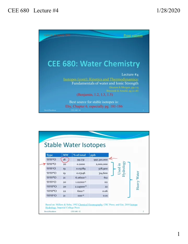
Stable Water Isotopes
Type MW % of total ppb
1H1H16O
18 99.731 997,310,000
1H1H18O
20 0.2000 2,000,000
1H1H17O
19 0.03789 378,900
1H2H16O
19 0.03146 314,600
1H2H18O
21 6.116x10‐5 612
1H2H17O
20 1.122x10‐5 112
2H2H16O
20 2.245x10‐6 22
2H2H18O
22 6x10‐9 0.06
2H2H17O
21 1x10‐9 0.01
David Reckhow CEE 680 #2 2
Based on: Millero & Sohn, 1992 Chemical Oceanography, CRC Press; and Gat, 2010 Isotope Hydrology, Imperial College Press
Heavy Water Used in Hydrology