a brief summary of isotopes and fractionation
play

A brief summary of isotopes and fractionation 1. Isotopes are - PDF document

A brief summary of isotopes and fractionation 1. Isotopes are chemically identical, but mechanically different. 2. Different masses lead to different bond frequencies... = 1 Hooke's Law 2 3. ...which lead to different zero-point


  1. A brief summary of isotopes and fractionation 1. Isotopes are chemically identical, but mechanically different. 2. Different masses lead to different bond frequencies... ν = 1 κ Hooke's Law µ 2 π 
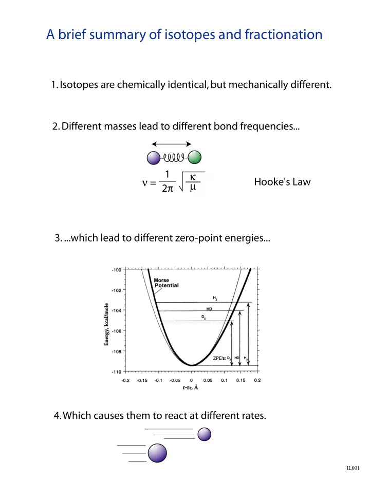
3. ...which lead to different zero-point energies... 4. Which causes them to react at different rates. IL001

  2. Isotope Effects verus Fractionation 12 C 12 C 13 C ∆ 13 C An Isotope Effect Fractionation causes R P + Q For equilibrium rxns:� � HDO + H 2 H 2 O + HD [H 2 O][HD] α = R H2 / R H2O = 0.30 = 0.30 E.I.E. = K eq =[HDO][H 2 ] (i.e., -700‰!) + e - For nonequilibrium rxns:� 2H 2 O� � � 2H 2 + O 2 2HDO� � � 2HD + O 2 K.I.E. = K H / K D = 2.7 α = R H2 / R H2O = 0.37 (but not consistently applied!) IL002

  3. Delta Notation Introduced in 1948 by Harold Urey, partly for conciseness and partly to emphasize that we measure relative isotope ratios very accurately, but absolute isotope ratios only poorly. All delta values are relative. Defining accuracy can be a bit tricky. Slight confusion over its definition: R samp - R std ∆ R δ = δ = 10 3 or R std R std in ‰ units ‰ implies factor of 10 3 Good: delta values can usually be added linearly, making mass balance equations straightforward (including blank correction) n t δ t = n 1 δ 1 + n 2 δ 2 + ... Bad: delta values are only linear over a small range of absolute abundance so be careful with hydrogen and isotopic labels 200 1,200,000 100 δ 13 C (‰) 800,000 0 400,000 S MOW -100 0 -1,000 -200 0.0 0.5 1.0 0.008 0.010 0.012 0.014 13 C fractional abundance 13 C fractional abundance IL004

  4. Measures of Fractionation α ε symbol: ∆ ∆ δ A +1000 ( α -1)10 3 defn. 1000ln( α ) δ A - δ B δ B +1000 all used for: kinetic equil. equil. 0.8 -200.0 -223.1 -250.0 0.900 -100.0 -105.4 -111.1 0.980 -20.0 -20.2 -20.4 0.990 -10.0 -10.1 -10.1 1.000 0.0 0.0 0.0 1.010 10.0 10.0 9.9 1.020 20.0 19.8 19.6 1.100 100.0 95.3 90.9 1.200 200.0 182.3 166.7 12 for constant α =1.100 11 B A - δ 10 δ 9 8 -200 0 200 δ A remember delta scale is not linear! IL006

  5. Equilibrium Fractionations Fractionations can exist between different phases of the same compound, as well as between different compounds Equilibrium isotope effects are usually temperature dependent but pressure independent. Fractionations form basis for thermometry. "Normal" EIE means heavy isotope accumulates in stronger bond, or light isotope is more volatile, and fractionation decreases with T. There are exceptions. Equil. isotope effects are difficult to measure direclty, but can be predicted from calculations, at least for simple molecules. Equilibrium fractionations can be measured directly by equilibrating materials at constant T. IL005

  6. PA1001 VAN DER LAAN ET AL.: LATE MIOCENE STABLE ISOTOPE RECORDS PA1001 Cyclostratigraphy and magnetostratigraphy of Ain el Beida with planktonic and benthic 18 O Figure 2. and sedimentation rate. Tuning of the sedimentary cyclicity to the 65 N summer insolation and precession curves of the La93 (1,1) astronomical solution [ Laskar et al. , 1993]. Magnetostratigraphy is based on Krijgsman et al. [2004]. Time-equivalent lithologic units in the Mediterranean are shown at the right-hand side of the figure [after Krijgsman et al. , 2001]. The initiation of the MSC at 5.96 Ma is indicated by an arrow.

  7. Kinetic Fractionations H 2 DC -- D CH 2 D 2 D 2 HC -- H energy CH 2 DCl CHD 2 Cl α reaction coordinate Kinetic isotope effects can be rationalized in terms of the potential energy barrier of the reaction. The lower the barrier, the faster the reaction Kinetic isotope effects are usually independent of both temperature and pressure. KIE's are typically constant for a particular reaction. "Normal" KIE means light isotope reacts more rapidly. There are very few known exceptions, and nearly all involve D/H. Kinetic isotope effects are easy to measure directly, but cannot generally be predicted from theory. Kinetic fractionations can be tricky to measure in natural systems because fractionation often depends on reaction yield. IL012

  8. Open System Fractionation "Open" means that reactant is available in unlimited supply. With only one product, isotopic composition of product is constant. ε P/R δ P = δ R + ε P/R R P With two or more products, isotopic composition depends on relative yield of each product. Isotopic mass balance must be maintained (what goes in must come out). Q Reaction R Chamber P Q A = α P/R / α Q/R A Isotope ratio = ε P/R − ε Q/R P 0 0.5 1.0 yield of P IL013

  9. Example of Open System Fractionation At the broadest level, inputs to the global C cycle (weathering, volcanism) must match outputs (buried carbonate and organic matter) δ a carbonate carbon δ i CO 2 ε TOC biosphere inputs δ o organic carbon δ i = f o δ o + (1- f o ) δ a ε TOC = δ a − δ o δ i = f o (δ a − ε TOC ) + δ a − f o δ a = δ a − f o ε TOC δ a − δ i f o = ε TOC Hayes, Strauss, & Kaufman (1999) Chemical Geology, 161:103-125. Thus we can interpret f o , an important operating condition of the global carbon cycle (and biosphere) from measurements of only 3 quantities.

  10. Closed System Fractionation If the reactant is in limited supply, its composition will change as it is consumed by the reaction. Fractionation R P Isotope Effect Fractionation between pooled product and unconsumed reactant is variable Isotope ratio A = f (yield, isotope effect) A R Fractionation between instantaneously B P' forming product and unconsumed reactant is constant P B = f (isotope effect) 0 0.5 1.0 yield of P (= f ) ε = ( δ rf - δ ro ) / ln(1- f ) Fractionation can be due either to kinetic or equilibrium isotope effects (if P is continually removed). The latter case is often called "Rayleigh Distillation". IL014

  11. Fractionation in Precipitation δ D = -128‰ δ D = -198‰ δ D = -76‰ f = 0.5 f = 0.8 α eq = 0.924 δ D = -53‰ (25°C) δ D = -122‰ δ D = 0‰ all equilibria at 25°C Ocean Precipitation becomes D-enriched as more rain condenses (farther from the ocean) δ D = -145‰ δ D = -237‰ δ D = -76‰ f = 0.5 f = 0.8 α eq = 0.900 (5°C) α eq = 0.924 δ D = -45‰ (25°C) δ D = -137‰ δ D = 0‰ clouds at 5°C Ocean The effect is exaggerated at colder temperatures because the liquid/vapor fractionation is larger IL016

Download Presentation
Download Policy: The content available on the website is offered to you 'AS IS' for your personal information and use only. It cannot be commercialized, licensed, or distributed on other websites without prior consent from the author. To download a presentation, simply click this link. If you encounter any difficulties during the download process, it's possible that the publisher has removed the file from their server.

Recommend


More recommend