
SLIDE 1
1
- Sequence of instructions that in the absence of
- ther activities is continuously executed by the
processor until completion.
Task model
Task i
activation time Ci start time finishing time t ai si fi computation time Response time Ri
- It is a task characterized by a timing constraint on
its response time, called deadline:
Real-Time Task
relative deadline Di
t ai si fi response time Ri di absolute deadline (di = ai + Di)
A real-time task i is said to be feasible if it completes within its absolute deadline, that is, if fi di, o equivalently, if Ri Di i
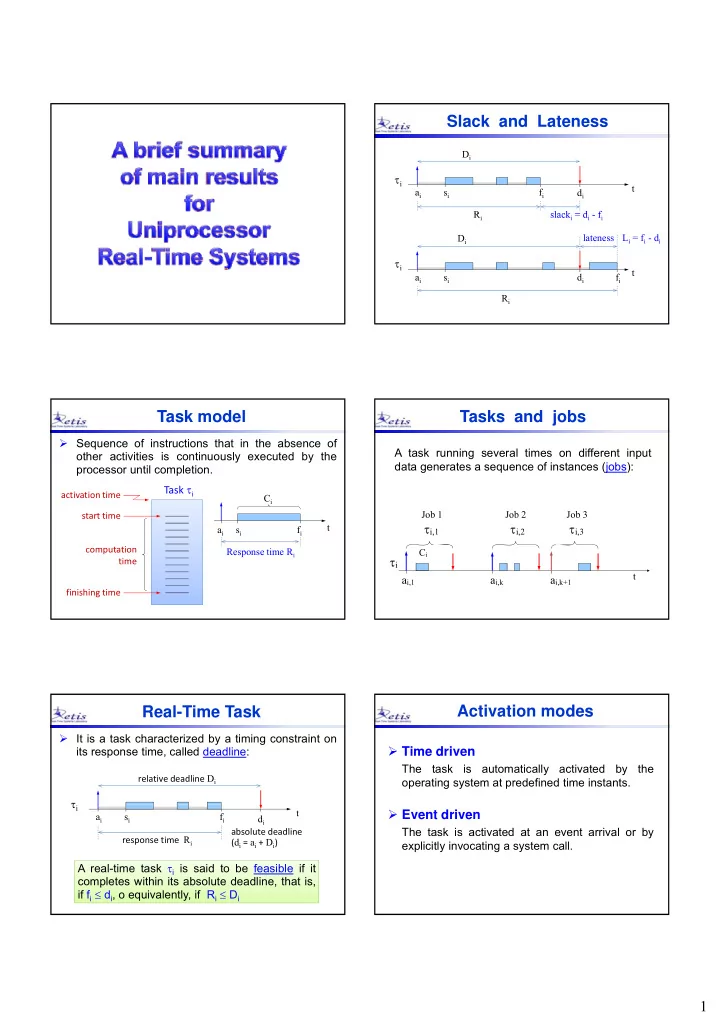
Slack and Lateness
t ai si fi R di Di
i
slack = d f Ri slacki = di - fi t ai si fi Ri di Di
i
lateness Li = fi - di
Tasks and jobs
A task running several times on different input data generates a sequence of instances (jobs): ai,k ai,k+1
t
i
Ci
ai,1
Job 1
i,1 i,2 i,3
Job 2 Job 3
Activation modes
- Time driven
The task is automatically activated by the
- perating system at predefined time instants.
- Event driven