
SLIDE 1
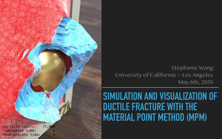
SIMULATION AND VISUALIZATION OF DUCTILE FRACTURE WITH THE MATERIAL POINT METHOD (MPM)
Stephanie Wang University of California — Los Angeles May 6th, 2020
Particle count: 77,000 Simulation time: 2 Mesh-process time: 5
SIMULATION AND VISUALIZATION OF DUCTILE FRACTURE WITH THE MATERIAL - - PowerPoint PPT Presentation
Stephanie Wang University of California Los Angeles May 6th, 2020 SIMULATION AND VISUALIZATION OF DUCTILE FRACTURE WITH THE MATERIAL POINT METHOD (MPM) Particle count: 77,000 Simulation time: 2 Mesh-process time: 5
Stephanie Wang University of California — Los Angeles May 6th, 2020
Particle count: 77,000 Simulation time: 2 Mesh-process time: 5
▸ PhD Advisor: Joseph Teran, UCLA ▸ Xuchen Han, UCLA ▸ Qi Guo, UCLA ▸ Mengyuan Ding, UCLA ▸ Steven Gagniere, UCLA ▸ Leyi Zhu, University of Science and Technology of
China
▸ Theodore Gast, JIXIE EFFECTS (UCLA) ▸ Chenfanfu Jiang, University of Pennsylvania (UCLA)
Particle count: 60,000 Simulation time: 11 Mesh-process time: —-
Particle count: 60,000 Simulation time: 11 Mesh-process time: 5
Particle count: 207,000 Simulation time: 16 Mesh-process time: 13
Particle count: 207,000 Simulation time: 16 Mesh-process time: 13
Particle count: 207,000 Simulation time: 16 Mesh-process time: 13
▸ Material Point Method (MPM) ▸ Grid-particle transfer ▸ Force computation ▸ Simulation and visualization of ductile fracture ▸ Yield surfaces ▸ Mesh-processing ▸ Discussion
Particle count: 200,000 Simulation time: 35 Mesh-process time: 16
▸ Particles for state ▸ Grid for computations ▸ Interpolation between particles and grid ▸ Similar to FEM: Vertices for state, Mesh for computations
MATERIAL POINT METHOD (MPM)
mn
i = TransferP2G(mp)
vn
i = TransferP2G(vn p)
f n
i = ComputeForce()
˜ vn+1
i
= vn
i + ∆t
mn
i
f n
i
vn+1
p
= TransferG2P(˜ vn+1
i
) xn+1
p
= xn
p + ∆tvn+1 p
⇐ Beware!
MATERIAL POINT METHOD (MPM)
mp vn
i
xn+1
p
notation meaning when where position after forces particle velocity before forces grid mass never changes particle
mn
i = TransferP2G(mp)
vn
i = TransferP2G(vn p)
f n
i = ComputeForce()
˜ vn+1
i
= vn
i + ∆t
mn
i
f n
i
vn+1
p
= TransferG2P(˜ vn+1
i
) xn+1
p
= xn
p + ∆tvn+1 p
⇐ Beware!
MATERIAL POINT METHOD (MPM)
mp vn
i
xn+1
p
notation meaning when where position after forces particle velocity before forces grid mass never changes particle
PARTICLE-GRID TRANSFER
▸ Compactly supported kernel function ▸ Spline: C1 (C2) piecewise-polynomial
ˆ N(x)
Quadratic Cubic
▸ Tensor product: ▸ Compute weights: ▸ Partition of unity ▸ Barycentric embedding ▸ Conservation of momenta, non-increasing energy
N(x) = ˆ N(x) ˆ N(y) ˆ N(z)
PARTICLE-GRID TRANSFER
wn
ip = N(xn i xn p)
rwn
ip = rN(xn i xn p)
X
i
wn
ip = 1
X
i
wn
ipxn i = xn p
mn
i =
X
p
wn
ipmp
mn
i vn i =
X
p
wn
ipmpvn p
Mass Momentum
vn+1
p
= X
i
wn
ip˜
vn+1
i
PARTICLE-GRID TRANSFER
Kernel at particle Kernel at node
mn
i =
X
p
wn
ipmp
vn
i =
1 mn
i
X
p
wn
ipmpvn p
f n
i = ComputeForce()
˜ vn+1
i
= vn
i + ∆t
mn
i
f n
i
vn+1
p
= X
i
wn
ip˜
vn+1
i
xn+1
p
= xn
p + ∆tvn+1 p
mn
i =
X
p
wn
ipmp
Dn
p =
X
i
wn
ip(xn i − xn p)(xn i − xn p)T
vn
i =
1 mn
i
X
p
wn
ipmp(vn p + Bn p(Dn p)−1(xn i − xn p))
f n
i = ComputeForce()
˜ vn+1
i
= vn
i + ∆t
mn
i
f n
i
vn+1
p
= X
i
wn
ip˜
vn+1
i
Bn+1
p
= X
i
wn
ipvn i (xn i − xn p)T
xn+1
p
= xn
p + ∆tvn p
Particle In Cell (PIC) Affine Particle In Cell (APIC)
PARTICLE-GRID TRANSFER
▸ Particle In Cell (PIC): Harlow 1964 ▸ Fluid Implicit Particle (FLIP): Brackbill and Ruppel 1986 ▸ Affine Particle In Cell (APIC): Jiang et al. 2015 ▸ Rigid Particle In Cell (RPIC): Jiang et al. 2015 ▸ Polynomial Particle In Cell (PolyPIC): Fu et al. 2017 ▸ Extended Particle In Cell (XPIC): Hammerquist et al. 2017
PARTICLE-GRID TRANSFER
mn
i = TransferP2G(mp)
vn
i = TransferP2G(vn p)
f n
i = ComputeForce()
˜ vn+1
i
= vn
i + ∆t
mn
i
f n
i
vn+1
p
= TransferG2P(˜ vn+1
i
) xn+1
p
= xn
p + ∆tvn+1 p
⇐ Beware!
MATERIAL POINT METHOD (MPM)
mp vn
i
xn+1
p
notation meaning when where velocity before forces grid position after forces particle mass never changes particle
mn
i = TransferP2G(mp)
vn
i = TransferP2G(vn p)
f n
i = ComputeForce()
˜ vn+1
i
= vn
i + ∆t
mn
i
f n
i
vn+1
p
= TransferG2P(˜ vn+1
i
) xn+1
p
= xn
p + ∆tvn+1 p
⇐ Beware!
MATERIAL POINT METHOD (MPM)
mp vn
i
xn+1
p
notation meaning when where velocity before forces grid position after forces particle mass never changes particle
FORCE COMPUTATION
F
Xb Xa
x = Φ(X, t) F(X, t) = ∂Φ ∂X(X, t)
Ω0 Ωt
FORCE COMPUTATION
mesh-based forces: F per triangle particle-based forces: F per particle
Φ = X
e
V 0
e Ψ(Fe)
Φ = X
p
V 0
p Ψ(Fp)
FORCE COMPUTATION
▸ First Piola-Kirchoff stress ▸ Total potential energy ▸ ``F is a function of x” ▸ Energy is a function of x ▸ Force can be computed from x
P(F) = ∂Ψ ∂F(F)
Φ = X
p
V 0
p Ψ(Fp)
Fn+1
p
= I + ∆t X
i
vi(rωn
ip)T
! Fn
p
fi = − ∂Φ ∂xi fi = ∂Φ ∂xi = X
p
V 0
p
✓∂Ψ ∂F(Fp(x)) ◆ (Fn
p)T rωn ip
Fn
e =
X
q
xn
q rNq(Xe)T
FORCE COMPUTATION
▸ St. Venant Kirchhoff potential with Hencky strain ▸ (Easy for analytical plastic projection)
F = UΣVT ψ(F) = µtr((ln Σ)2) + λ 2 (tr(ln Σ))2 ∂ψ ∂F = U(2µΣ−1 ln Σ + λtr(ln Σ)Σ−1)VT
FORCE COMPUTATION
FORCE COMPUTATION
FORCE COMPUTATION
FORCE COMPUTATION
Φ = X
e
V 0
e Ψ(Fe)
Φ = X
e
V 0
e Ψ(Fe)
Fn
e =
X
q
xn
q rNq(Xe)T
Fn
e =
X
q
xn
q rNq(ξe)T
! X
q
XqrNq(ξe)T !−1
FORCE COMPUTATION
FORCE COMPUTATION
FORCE COMPUTATION
FORCE COMPUTATION
FORCE COMPUTATION
FORCE COMPUTATION
FORCE COMPUTATION
FORCE COMPUTATION
Φ = X
p
V 0
p Ψ(Fp)
Fn+1
p
= I + ∆t X
i
vi(rωn
ip)T
! Fn
p
FORCE COMPUTATION
Φ = X
e
V 0
e Ψ(Fe)
Fn
e =
X
q
xn
q rNq(Xe)T
f n
i =
X
q
ωn
iqf n q
Particle count: 4,000 Simulation time: 5 Mesh-process time: 0.2
▸ Constraining maximal principal stress ▸ Mode I yielding (tension) ▸ Softening rule
y(τ) = max
kuk=kvk=1 uT τv − τC ≤ 0
⌧ n+1
C
= ⌧ n
C + ↵
✓ max
kuk=kvk=1 uT ✏n+1v −
max
k˜ uk=k˜ vk=1 ˜
uT ✏tr˜ v ◆
YIELD SURFACES
Particle count: 130,000 Simulation time: 15 Mesh-process time: 8
▸ Constraining shear stress ▸ Mode II and III yielding (shear) ▸ Softening can be added
y(τ) = kτ tr(τ)IkF τC 0
YIELD SURFACES
τC/E = 0.5 τC/E = 0.7
τC/E = 1
Particle count: 60,000 Simulation time: 11 Mesh-process time: 4
Particle count: 60,000 Simulation time: 11 Mesh-process time: 5
MESH-PROCESSING
▸ Fracturing topology (that evolves with time) ▸ Extrapolate positions for the added vertices ▸ Smoothing crack surface to reduce mesh-dependent noise ▸ Advantage: per-frame post-process instead of per-time-step
treatment
MESH-PROCESSING
MESH-PROCESSING
MESH-PROCESSING
MESH-PROCESSING
MESH-PROCESSING
MESH-PROCESSING
duplicated vertices
MESH-PROCESSING
MESH-PROCESSING
MESH-PROCESSING
1 2 3 3 4 5 6
▸ Subdivided mesh ▸ Edge-stretching
cutting criterion
▸ Evolves with time
MESH-PROCESSING
MESH-PROCESSING
MESH-PROCESSING
MESH-PROCESSING
MESH-PROCESSING
MESH-PROCESSING
MESH-PROCESSING
MESH-PROCESSING
1 2 3
▸ Granular view ▸ Locally rigid motion ▸ Merging vertices
based on topology
3 4 5
MESH-PROCESSING
MESH-PROCESSING
1 2 3
▸ Collect all ever broken
edges
▸ Gauss-Siedel
smoothing
▸ Smooth only the
undeformed configuration
3 4 5
DISCUSSION
▸ Crack patterns can be affected by particle sampling density, mesh
topology, grid resolution
▸ Finding appropriate parameters for edge-stretching threshold and
crack smoothing iterations
▸ Exploring different yield surfaces and flow rules
NUMERICAL METHODS
Particle-based forces (grid velocity updated F) Mesh-based forces (mesh geometry updated F)
Delaunay mesh for visualization requires quality mesh for simulation has artificial fracture no artificial fracture 6-8 particles per cell 2 particles per cell automatic self-collision easy coupling with other MPM material
Small grid dx Large grid dx Lagrangian
Particle count: 8,000 Simulation time: 0.6 Post-process time: 0.5
Particle count: 2,290,000 Element count: 930,000 Simulation time: 50 Mesh-process time: 5
The work is supported by NSF CCF-1422795, ONR (N000141110719, N000141210834), DOD (W81XWH15-1-0147), Intel STC-Visual Computing Grant (20112360) as well as a gift from Adobe Inc.
Particle count: 5,500 - 77,000 Simulation time: 0.2 - 2 Mesh-process time: 0.3 - 5