Shaken braid arrangements and trees Olivier Bernardi - Brandeis - - PowerPoint PPT Presentation

Shaken braid arrangements and trees

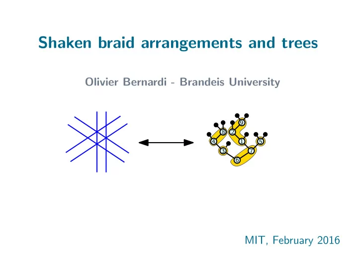
MIT, February 2016 Olivier Bernardi - Brandeis University

6 3 7 4 8 1 5 2 9

Shaken braid arrangements and trees

MIT, February 2016 Olivier Bernardi - Brandeis University

6 3 7 4 8 1 5 2 9 6 8 3 5 2 4 7 9 1

Hyperplane arrangements A hyperplane arrangement of dimension n is a finite collection of affine hyperplanes in Rn. Example: x1 x2

Hyperplane arrangements A hyperplane arrangement of dimension n is a finite collection of affine hyperplanes in Rn. The hyperplanes cut the space into regions. Example: x1 7 regions x2

Braid arrangement Def: The braid arrangement of dimension n has hyperplanes {xi − xj = 0} for all 0 ≤ i < j ≤ n.

Braid arrangement Example: n = 3 Def: The braid arrangement of dimension n has hyperplanes {xi − xj = 0} for all 0 ≤ i < j ≤ n. x1 x3 x2 x1 − x2 = 0 x1 − x3 = 0 x2 − x3 = 0

Braid arrangement Example: n = 3 Def: The braid arrangement of dimension n has hyperplanes {xi − xj = 0} for all 0 ≤ i < j ≤ n. x1 x3 x2 x1 − x2 = 0 x1 − x3 = 0 x2 − x3 = 0 n! regions

Shaken braid arrangements Def: Fix S ⊂ Z finite. The S-shaken braid arrangement AS(n) ⊂ Rn has hyperplanes {xi − xj = s} for all 0 ≤ i < j ≤ n, and all s ∈ S. We denote rS(n) = #regions of AS(n).

Shaken braid arrangements Def: Fix S ⊂ Z finite. The S-shaken braid arrangement AS(n) ⊂ Rn has hyperplanes {xi − xj = s} for all 0 ≤ i < j ≤ n, and all s ∈ S. x1 x3 x2 Example: S = {0, 1} and n = 3. rS(3) = 16 x1 − x2 = 0 x1 − x2 = 1 We denote rS(n) = #regions of AS(n).

Known relations with trees [Athanasiadis, Postnikov, Stanley,. . . ] Let B(n) be the set of rooted binary trees with n labeled nodes. 6 3 7 4 8 1 5 2 9 |B(n)| = Cat(n) × n! = (2n)! (n + 1)!

Catalan Shi Semi-order Linial Braid T ∈B(n) u v u > v u v u > w u v u < v u w u v u v u > v u w u v u > w u v u w T ∈B(n) s.t. T ∈B(n) s.t. T ∈B(n) s.t. T ∈B(n) s.t. Known relations with trees S ={−1, 0, 1} [Athanasiadis, Postnikov, Stanley,. . . ] S ={0, 1} S ={−1, 1} S ={1} S ={0} u v u > v

Catalan Shi Semi-order Linial Braid T ∈B(n) u v u > v u v u > w u v u < v u w u v u v u > v u w u v u > w u v u w T ∈B(n) s.t. T ∈B(n) s.t. T ∈B(n) s.t. T ∈B(n) s.t. Known relations with trees S ={−1, 0, 1} [Athanasiadis, Postnikov, Stanley,. . . ] S ={0, 1} S ={−1, 1} S ={1} S ={0}

“Why?” Ira Gessel

u v u > v

Catalan Shi Semi-order Linial Braid T ∈B(n) u v u > v u v u > v u v u > w u v u < v u w u v u v u > v u w u v u > w u v u w T ∈B(n) s.t. T ∈B(n) s.t. T ∈B(n) s.t. T ∈B(n) s.t. Known relations with trees S ={−1, 0, 1} [Athanasiadis, Postnikov, Stanley,. . . ] S ={0, 1} S ={−1, 1} S ={1} S ={0}

“Why?” Ira Gessel

u v u > v u1 u2 un u v u > v

Arrangements, trees, and discrete gas

Boxed trees

• T (m) = set of rooted (m+1)-ary trees with labeled nodes.

6 2 8 4 10 9 1 5 11 3 1 7 4 12 13

Boxed trees

• T (m) = set of rooted (m+1)-ary trees with labeled nodes.

6 2 8 4 10 9 1 5 11 3 1 7

• The last node among the children of u is denoted cadet(u).
• A cadet-sequence is any sequence of node (v1, . . . , vk) such

that vi+1 = cadet(vi).

4 12 13

Boxed trees

• T (m) = set of rooted (m+1)-ary trees with labeled nodes.

6 2 8 4 10 9 1 5 11 3 1 7

• A m-boxed tree is a tree in T (m) decorated with boxes

partitioning the nodes into cadet-sequences.

• The last node among the children of u is denoted cadet(u).
• A cadet-sequence is any sequence of node (v1, . . . , vk) such

that vi+1 = cadet(vi).

4 12 13

Main result Def: A S-boxed tree is a m-boxed tree such that each box satisfies ∀i < j, if (ci+ci+1+· · ·+cj−1) ∈ S ∪ {0} then vi < vj, if −(ci+ci+1+· · ·+cj−1) ∈ S then vi > vj. v1 v2 c1 ci cj Let S ⊂ Z. Let m = max(|s|, s ∈ S). vj vk m + 1 vi

Main result Def: A S-boxed tree is a m-boxed tree such that each box satisfies ∀i < j, if (ci+ci+1+· · ·+cj−1) ∈ S ∪ {0} then vi < vj, if −(ci+ci+1+· · ·+cj−1) ∈ S then vi > vj. Let S ⊂ Z. Let m = max(|s|, s ∈ S). Example: S = [−a .. m] with a ∈ {0, ..., m}

a<ci ≤m

v1 v2 vk vi

v1 <v2 < · · · <vk

Main result Def: A S-boxed tree is a m-boxed tree such that each box satisfies ∀i < j, if (ci+ci+1+· · ·+cj−1) ∈ S ∪ {0} then vi < vj, if −(ci+ci+1+· · ·+cj−1) ∈ S then vi > vj. Let S ⊂ Z. Let m = max(|s|, s ∈ S). Theorem: rS(n) =

• T ∈US(n)

(−1)n−#boxes, where US(n) is the set of S-boxed trees with n nodes,

Def: S is transitive if

• If a, b /

∈ S, with ab > 0, then a + b / ∈ S,

• If a, b /

∈ S, with ab < 0, then a − b / ∈ S,

• If 0, a /

∈ S, with a > 0, then −a / ∈ S. Corollary

Examples:

• Any subset of {−1, 0, 1}.
• Any interval of integers containing 1.
• S such that [−k; k] ⊆ S ⊆[−2k; 2k] for some k.

Def: S is transitive if

• If a, b /

∈ S, with ab > 0, then a + b / ∈ S,

• If a, b /

∈ S, with ab < 0, then a − b / ∈ S,

• If 0, a /

∈ S, with a > 0, then −a / ∈ S. Corollary

Def: S is transitive if

• If a, b /

∈ S, with ab > 0, then a + b / ∈ S,

• If a, b /

∈ S, with ab < 0, then a − b / ∈ S,

• If 0, a /

∈ S, with a > 0, then −a / ∈ S. Def: TS is set of trees in T (m) such that any v = cadet(u) satisfies Cond(S): if #left-siblings(v) / ∈ S ∪ {0} then u < v, if − #left-siblings(v) / ∈ S then u > v. Corollary v u #left-siblings(v)

Def: S is transitive if

• If a, b /

∈ S, with ab > 0, then a + b / ∈ S,

• If a, b /

∈ S, with ab < 0, then a − b / ∈ S,

• If 0, a /

∈ S, with a > 0, then −a / ∈ S. Corollary: If S is transitive, then rS(n) = |TS(n)| Def: TS is set of trees in T (m) such that any v = cadet(u) satisfies Cond(S): if #left-siblings(v) / ∈ S ∪ {0} then u < v, if − #left-siblings(v) / ∈ S then u > v. Corollary

Corollary Def: TS is set of trees in T (m) such that any v = cadet(u) satisfies Cond(S) : if #left-siblings(v) / ∈ S ∪ {0} then u < v, if − #left-siblings(v) / ∈ S then u > v. Corollary: If S is transitive, then rS(n) = |TS(n)| Example: S = {−2, −1, 0, 1, 3} v u ⇒ u < v u ⇒ u > v v Cond(S) :

Corollary Example: Catalan If S = [−m..m], then TS(n) = T (m)(n). Semiorder If S[−m..m] \ {0}, then Cond(S)=“cadets with 0 left-siblings are less than parent”. Shi If S = [−a..m] with a ∈ {0, . . . , m}, then Cond(S)=“cadets with > a left-siblings are less than parent”. Linial If S[−a..m] \ {0} with a ∈ {0, . . . , m}, then Cond(S)=“cadets with 0 or > a left-siblings are less than parent”. Def: TS is set of trees in T (m) such that any v = cadet(u) satisfies Cond(S) : if #left-siblings(v) / ∈ S ∪ {0} then u < v, if − #left-siblings(v) / ∈ S then u > v. Corollary: If S is transitive, then rS(n) = |TS(n)|

Proof of corollary. Locality: For S transitive a m-boxed tree is S-boxed if and only if ∀i < j, if ci ∈ S ∪ {0} then vi < vi+1, if −ci ∈ S then vi > vi+1.

v1

v2 ci vi

+ 1

vk vi

Proof of corollary. Remark: For v = cadet(u) u, v satisfies Cond(S) ⇐ ⇒ u and v cannot be in same S-box. Locality: For S transitive a m-boxed tree is S-boxed if and only if ∀i < j, if ci ∈ S ∪ {0} then vi < vi+1, if −ci ∈ S then vi > vi+1.

Proof of corollary. Remark: For v = cadet(u) u, v satisfies Cond(S) ⇐ ⇒ u and v cannot be in same S-box. Locality: For S transitive a m-boxed tree is S-boxed if and only if ∀i < j, if ci ∈ S ∪ {0} then vi < vi+1, if −ci ∈ S then vi > vi+1. Sign-reversing involution: rS(n) =

• T ∈US,

satisfying Cond(S)

(−1)n−#boxes +

• T ∈US,

not satisfying Cond(S)

(−1)n−#boxes |TS(n)| Must have a different box around each node. Merge/split box at v = cadet(u) not satisfying Cond(S).

Proof of Theorem x1 x3 x2 Zaslavky formula + Mayers’ clusters Decomposition in runs

6 3 7 4 8 1 5 2 9

Zaslavky formula + Mayers’ clusters

6 1 4 2 7 9 5 3 8

discrete gas model

Lemma 1: rS(n) =

• G=([n],E)

(−1)e+c−n|WS(G)|, where e=#edges, c=#components, n=#vertices, and WS(G)= set of tuples (x1, . . . , xn) such that

• ∀{i, j} ∈ E with i < j,

xi − xj ∈ S,

• ∀i ∈ [n] smallest in its component,

xi = 0.

Lemma 1: rS(n) =

• G=([n],E)

(−1)e+c−n|WS(G)|, where e=#edges, c=#components, n=#vertices, and WS(G)= set of tuples (x1, . . . , xn) such that

• ∀{i, j} ∈ E with i < j,

xi − xj ∈ S,

• ∀i ∈ [n] smallest in its component,

xi = 0. Proof: Zaslavsky formula: For any arrangement A ⊂ Rn, #regions of A =

• B⊆A, B=∅

(−1)|B|+dim( B)−n. Example: # regions = 1 + 4 + 5 − 1 = 9

|B| = 0 |B| = 1 |B| = 3 |B| = 2

A

Lemma 1: rS(n) =

• G=([n],E)

(−1)e+c−n|WS(G)|, where e=#edges, c=#components, n=#vertices, and WS(G)= set of tuples (x1, . . . , xn) such that

• ∀{i, j} ∈ E with i < j,

xi − xj ∈ S,

• ∀i ∈ [n] smallest in its component,

xi = 0. x1 x3 x2 Proof: AS(n) B

x1 −x2 = 0 x2 −x3 = 1 3 1 2

(0, 0, −1) B

Lemma 1: rS(n) =

• G=([n],E)

(−1)e+c−n|WS(G)|, where e=#edges, c=#components, n=#vertices, and WS(G)= set of tuples (x1, . . . , xn) such that

• ∀{i, j} ∈ E with i < j,

xi − xj ∈ S,

• ∀i ∈ [n] smallest in its component,

xi = 0. x1 x3 x2 Proof: AS(n) B

x1 −x2 = 0 x2 −x3 = 1

B (G , (x1, . . . , xn)) G = graph with vertices [n] and edges {i, j} s.t. ∃ {xi − xj = s} ∈ B. (x1, . . . , xn)= point in B s.t. ∀i ∈ [n] smallest in its component, xi = 0.

3 1 2

(0, 0, −1) B

Lemma 1: rS(n) =

• G=([n],E)

(−1)e+c−n|WS(G)|, where e=#edges, c=#components, n=#vertices, and WS(G)= set of tuples (x1, . . . , xn) such that

• ∀{i, j} ∈ E with i < j,

xi − xj ∈ S,

• ∀i ∈ [n] smallest in its component,

xi = 0. x1 x3 x2 Proof: AS(n) B

x1 −x2 = 0 x2 −x3 = 1

B (G , (x1, . . . , xn)) G = graph with vertices [n] and edges {i, j} s.t. ∃ {xi − xj = s} ∈ B. (x1, . . . , xn)= point in B s.t. ∀i ∈ [n] smallest in its component, xi = 0. ⇒ rS(n) =

• B⊆AS(n), B=∅

(−1)|B|+dim( B)−n =

• G=([n],E),

(x1,..,xn)∈WS (G)

(−1)e+c−n.

Def: ZS,δ(n) = {(x1, . . . , xn) ∈ [δ]n | ∀i < j, xi − xj / ∈ S}. Example: (4, 13, 19, 13, 15, 3, 12, 21, 7) is in Z{−1,2},22(9).

Def: ZS,δ(n) = {(x1, . . . , xn) ∈ [δ]n | ∀i < j, xi − xj / ∈ S}.

1 6 2 δ = 22 1 4 2 7 9 5 3 8

Example: (4, 13, 19, 13, 15, 3, 12, 21, 7) is in Z{−1,2},22(9).

“discrete gas with potential given by S” Pressure: P = kT δ log

• n

|ZS,δ(n)| tn n!

Lemma 2: log (R(t)) = lim

δ→∞ −1

δ log(ZS,δ(−t)), Def: ZS,δ(n) = {(x1, . . . , xn) ∈ [δ]n | ∀i < j, xi − xj / ∈ S}. where R(t) =

• n≥0

rS(n)tn n!, and ZS,δ(t) =

• n≥0

|ZS,δ(n)|tn n!.

Lemma 2: log (R(t)) = lim

δ→∞ −1

δ log(ZS,δ(−t)), Proof:

• |ZS,d(n)|

=

• x1,...,xn∈[δ]
• i<j

1xi−xj /

∈S

=

• x1,...,xn∈[δ]
• i<j

(1 − 1xi−xj∈S) =

• x1,...,xn∈[δ]
• G=([n],E)

(−1)e

• {i,j}∈E, i<j

1xi−xj∈S =

• G=([n],E)

(−1)e

• x1,...,xn∈[δ]
• {i,j}∈E, i<j

1xi−xj∈S =

• G=([n],E)

(−1)e|WS,δ(G)|, where WS,δ(G)={(x1, . . . , xn) ∈ [δ]n | ∀{i, j} ∈ E, with i < j, xi−xj ∈ S}. Def: ZS,δ(n) = {(x1, . . . , xn) ∈ [δ]n | ∀i < j, xi − xj / ∈ S}.

Lemma 2: log (R(t)) = lim

δ→∞ −1

δ log(ZS,δ(−t)), Def: ZS,δ(n) = {(x1, . . . , xn) ∈ [δ]n | ∀i < j, xi − xj / ∈ S}. Proof:

• |ZS,d(n)|

=

• G=([n],E)

(−1)e|WS,δ(G)|, where WS,δ(G)={(x1, . . . , xn) ∈ [δ]n | ∀{i, j} ∈ E, with i < j, xi−xj ∈ S}

• Exponential formula:

= ⇒ log(RS(t))=

• G connected graph

(−1)e+c−v|WS(G)|tv v! log(ZS,δ(t))=

• G connected graph

(−1)e|WS,δ(G)|tv v! RS(t)=

• G graph

(−1)e+c−v|WS(G)|tv v! ZS,δ(t)=

• G graph

(−1)e|WS,δ(G)|tv v!

Lemma 2: log (R(t)) = lim

δ→∞ −1

δ log(ZS,δ(−t)), Def: ZS,δ(n) = {(x1, . . . , xn) ∈ [δ]n | ∀i < j, xi − xj / ∈ S}. Proof:

• |ZS,d(n)|

=

• G=([n],E)

(−1)e|WS,δ(G)|, where WS,δ(G)={(x1, . . . , xn) ∈ [δ]n | ∀{i, j} ∈ E, with i < j, xi−xj ∈ S}

• If G connected, then lim

δ→∞

1 δ |WS,δ(n)| = |WS(G)|, where WS(G)={(x1, . . . , xn) ∈ Zn | ∀{i, j} ∈ E, with i < j, xi−xj ∈ S, and x1 = 0}

• Exponential formula:

log(RS(t))=

• G connected graph

(−1)e+c−v|WS(G)|tv v!, log(ZS,δ(t))=

• G connected graph

(−1)e|WS,δ(G)|tv v!,

Lemma 3: ZS,δ(t) = US(t)−m−δ−2 U •

S(t)

Def: ZS,δ(n) = {(x1, . . . , xn) ∈ [δ]n | ∀i < j, xi − xj / ∈ S}. where US(t) =

• T S-boxed tree

(−1)#boxes tv v!, and U •

S(t) =related series.

Lemma 3: ZS,δ(t) = US(t)−m−δ−2 U •

S(t)

Proof: Def: ZS,δ(n) = {(x1, . . . , xn) ∈ [δ]n | ∀i < j, xi − xj / ∈ S}.

1 6 2 δ 1 4 2 7 9 5 3 8

S = {−1, 2}

Lemma 3: ZS,δ(t) = US(t)−m−δ−2 U •

S(t)

Proof: Def: ZS,δ(n) = {(x1, . . . , xn) ∈ [δ]n | ∀i < j, xi − xj / ∈ S}.

1 6 2 δ ρ1 ρ2 ρ3 ρ4 1 4 2 7 9 5 3 8

S = {−1, 2}

>m >m >m

Lemma 3: ZS,δ(t) = US(t)−m−δ−2 U •

S(t)

Proof: Def: ZS,δ(n) = {(x1, . . . , xn) ∈ [δ]n | ∀i < j, xi − xj / ∈ S}.

1 6 2 δ ρ1 ρ2 ρ3 ρ4 1 4 2 7 9 5 3 8 6 1

S = {−1, 2}

9 4 2 7 5 3 8

runs

Lemma 3: ZS,δ(t) = US(t)−m−δ−2 U •

S(t)

Proof: Def: ZS,δ(n) = {(x1, . . . , xn) ∈ [δ]n | ∀i < j, xi − xj / ∈ S}.

1 6 2 δ ρ1 ρ2 ρ3 ρ4 1 4 2 7 9 5 3 8

positions

6 1

S = {−1, 2}

9 4 2 7 5 3 8

δ + m − width(ρ1) − · · · − width(ρr) r

• runs

Lemma 3: ZS,δ(t) = US(t)−m−δ−2 U •

S(t)

Proof: Def: ZS,δ(n) = {(x1, . . . , xn) ∈ [δ]n | ∀i < j, xi − xj / ∈ S}.

1 6 2 δ ρ1 ρ2 ρ3 ρ4 1 4 2 7 9 5 3 8

positions

6 1

S = {−1, 2}

9 4 2 7 5 3 8

δ + m − width(ρ1) − · · · − width(ρr) r

• δ =−m−1−γ < 0

(−1)rγ + r + width(ρ1) + · · · + width(ρr) r

• (−1)r

γ ordered trees, r nodes with width(ρ1) + 1, . . . , width(ρr) + 1 children

runs polynomial in δ

Lemma 3: ZS,δ(t) = US(t)−m−δ−2 U •

S(t)

Proof: Def: ZS,δ(n) = {(x1, . . . , xn) ∈ [δ]n | ∀i < j, xi − xj / ∈ S}.

1 6 2 δ ρ1 ρ2 ρ3 ρ4 1 4 2 7 9 5 3 8

positions

6 1

S = {−1, 2}

9 4 2 7 5 3 8

δ + m − width(ρ1) − · · · − width(ρr) r

• δ =−m−1−γ < 0

(−1)rγ + r + width(ρ1) + · · · + width(ρr) r

• (−1)r

γ ordered trees, r nodes with width(ρ1) + 1, . . . , width(ρr) + 1 children

runs

6 1 9 4 2 7 5 3 8

S-boxed trees! polynomial in δ

Summary of proof

6 3 7 4 8 1 5 2 9

log (RS(t)) = lim

δ→∞ −1

δ log(ZS,δ(−t)) = lim

δ→∞ −1

δ log(US(−t)−δ−m−2U •

S(−t)) = log (US(−t))

RS(t) US(t) ZS,δ(t) Lemma 1+2 Lemma 3

6 8 3 5 2 4 7 9 1

Extensions Characteristic polynomial, Tutte polynomial of AS(n): χS(q, t) :=

• χAS(n)(q)tn

n! = R(−t)−q PS(q, y, t) :=

• PAS(n)(q, y)tn

n! = R(y, −t)−q

Extensions Multishaken braid arrangements: A(Si,j)1≤i<j≤n ⊂ Rn with hyperplanes {xi − xj ∈ Si,j} Characteristic polynomial, Tutte polynomial of AS(n): χS(q, t) :=

• χAS(n)(q)tn

n! = R(−t)−q PS(q, y, t) :=

• PAS(n)(q, y)tn

n! = R(y, −t)−q

Direct bijective approach for S ⊆ {−1, 0, 1}

Catalan configurations Warm up: Braid arrangement x1 x3 x2

x1 − x2 = 0 x2 − x3 = 0 x1 − x3 = 0 (x1, x2, x3) x3 x1 x2

Catalan configurations x1 x3 x2

x1 − x2 = 0 x1 − x2 = 1 (x1, x2, x3) x3 x1 x2 x3 x1 x2 x1+1 x3+1 x2+1

S = {−1, 0, 1}

x1 − x2 = −1

Catalan configurations x1 x3 x2

x1 − x2 = 0 x1 − x2 = 1 (x1, x2, x3) x3 x1 x2 x3 x1 x2 x1+1 x3+1 x2+1

S = {−1, 0, 1}

x1 − x2 = −1 3 1 2 n!Cat(n)

Bijection: Catalan configurations ← → binary trees

3 1 4 2 5

3 5 1 2 4

Shi/SO/Linial regions as equivalence class of Catalan regions

• Shi moves (S = {0, 1}):

i j j i if i < j

• Semi-order moves (S = {−1, 1}):

i j j i

• Linial moves (S = {1}) = Shi moves + semi-order moves

Definition:

Shi/SO/Linial regions as equivalence class of Catalan regions

• Shi moves (S = {0, 1}):

i j j i if i < j

• Semi-order moves (S = {−1, 1}):

i j j i

• Linial moves (S = {1}) = Shi moves + semi-order moves

Definition: Remark: Shi/SO/Linial regions are in bijection with equivalence classes of the Catalan configurations under Shi/SO/Linial moves.

Shi/SO/Linial regions as equivalence class of Catalan regions Definition: Order on Catalan configurations: C < C′ if the first place where they differ is either

• ց in C and ր in C′,
• ր in both, but label in C < label in C′.

Remark: Shi/SO/Linial regions are in bijection with configurations which are maximal in their equivalence class.

x1 x3 x2

123 132 312 213 231 321 3 2 1 2 3 1 1 2 3 1 3 2 2 1 3 3 1 2 1 2 3 1 3 2 2 3 1 3 2 1 3 1 2 2 1 3 1 2 3 1 3 2 2 3 1 2 1 3 3 1 2 3 2 1 1 3 2 2 3 1 3 2 1 1 2 3 3 1 2 2 1 3 A B A B B A A A A A A B B B A+B A A A A A+B A+B A+B A+B A+B A+B B B B

A=Semi-order max B=Shi max

Shi/SO/Linial regions as equivalence class of Catalan regions Definition: Order on Catalan configurations: C < C′ if the first place where they differ is either

• ց in C and ր in C′,
• ր in both, but label in C < label in C′.

Claim: Catalan configuration are Shi/SO/Linial-maximal if and

• nly if they are locally maximal: cannot increase by a single move.

Shi/SO/Linial regions as equivalence class of Catalan regions Definition: Order on Catalan configurations: C < C′ if the first place where they differ is either

• ց in C and ր in C′,
• ր in both, but label in C < label in C′.

Corollary:

• Shi regions are in bijection with configurations such that
• SO regions are in bijection with configurations such that
• Linial regions are in bijection with configurations such that

Claim: Catalan configuration are Shi/SO/Linial-maximal if and

• nly if they are locally maximal: cannot increase by a single move.

⇒ i > j j i ⇒ i > j j i i j ⇒ i > j i j ⇒ i > j and

Bijection: Catalan configurations ← → Trees

a b d e c

a

1 2

b a

2 1 3

b a

2 3

b a

3

c

2 4

b a

3

c

2 4

d

5

b a

3

c

4

d

5

b a c

4

d

5

b a c

4

d

5

e b a c d e

6

Φ b a c d

5

e

6

a

Bijection: Catalan configurations ← → Trees Claim: i j k i j k i j k i j k Φ Φ Φ Φ i j k i j i k i

Bijection: Catalan configurations ← → Trees Corollary:

• Shi regions are in bijection with trees such that
• SO regions are in bijection with trees such that
• Linial regions are in bijection with trees such that

u v u v u v u v and ⇒ u > v ⇒ u > v ⇒ u > v ⇒ u > v

x1 x3 x2 1 2 3 3 1 2 2 3 1 2 1 3 1 3 2 3 2 1 1 3 2 1 2 3 2 3 1 3 2 1 3 1 2 2 1 3 1 2 3 1 3 2 2 1 3 2 3 1 3 2 1 3 3 3 3 1 2 1 2 3 2 1 3 3 1 2 1 3 2 2 3 1 3 2 1 1 2 3 1 3 2 3 1 2 2 1 3 2 3 1 3 2 1 A A A+B A A+B B B B A A A A A A+B A A+B A+B B A B A B B A A+B B B B A+B

A=Semi-order B=Shi

Thanks.

6 3 7 4 8 1 5 2 9 6 8 3 5 2 4 7 9 1