
SLIDE 1
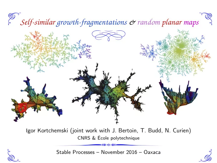
Self-similar growth-fragmentations & random planar maps
Igor Kortchemski (joint work with J. Bertoin, T. Budd, N. Curien)
CNRS & École polytechnique
Self-similar growth-fragmentations & random planar maps Igor - - PowerPoint PPT Presentation
Self-similar growth-fragmentations & random planar maps Igor Kortchemski (joint work with J. Bertoin, T. Budd, N. Curien) CNRS & cole polytechnique Stable Processes November 2016 Oaxaca Planar maps BienaymGaltonWatson
CNRS & École polytechnique
Planar maps Bienaymé–Galton–Watson trees Level sets of random maps
Igor Kortchemski Growth-fragmentations & random planar maps 1 / 2016
Planar maps Bienaymé–Galton–Watson trees Level sets of random maps
Igor Kortchemski Growth-fragmentations & random planar maps 1 / 2016
Planar maps Bienaymé–Galton–Watson trees Level sets of random maps
Igor Kortchemski Growth-fragmentations & random planar maps 1 / 2016
Planar maps Bienaymé–Galton–Watson trees Level sets of random maps
Igor Kortchemski Growth-fragmentations & random planar maps 1 / 2016
Planar maps Bienaymé–Galton–Watson trees Level sets of random maps
Igor Kortchemski Growth-fragmentations & random planar maps 1 / 2016
Planar maps Bienaymé–Galton–Watson trees Level sets of random maps
scaling limit
Igor Kortchemski Growth-fragmentations & random planar maps 1 / 2016
Planar maps Bienaymé–Galton–Watson trees Level sets of random maps
scaling limit
Igor Kortchemski Growth-fragmentations & random planar maps 1 / 2016
Planar maps Bienaymé–Galton–Watson trees Level sets of random maps
scaling limit scaling limit
Igor Kortchemski Growth-fragmentations & random planar maps 1 / 2016
Planar maps Bienaymé–Galton–Watson trees Level sets of random maps
scaling limit
Igor Kortchemski Growth-fragmentations & random planar maps 1 / 2016
Planar maps Bienaymé–Galton–Watson trees Level sets of random maps
n→∞
Igor Kortchemski Growth-fragmentations & random planar maps 2 / 2016
Planar maps Bienaymé–Galton–Watson trees Level sets of random maps
n→∞
Igor Kortchemski Growth-fragmentations & random planar maps 2 / 2016
Planar maps Bienaymé–Galton–Watson trees Level sets of random maps
n→∞
Igor Kortchemski Growth-fragmentations & random planar maps 2 / 2016
Planar maps Bienaymé–Galton–Watson trees Level sets of random maps
n→∞
Igor Kortchemski Growth-fragmentations & random planar maps 2 / 2016
Planar maps Bienaymé–Galton–Watson trees Level sets of random maps
n→∞
Igor Kortchemski Growth-fragmentations & random planar maps 2 / 2016
Planar maps Bienaymé–Galton–Watson trees Level sets of random maps
n→∞
Igor Kortchemski Growth-fragmentations & random planar maps 2 / 2016
Planar maps Bienaymé–Galton–Watson trees Level sets of random maps
Igor Kortchemski Growth-fragmentations & random planar maps 3 / 2016
Planar maps Bienaymé–Galton–Watson trees Level sets of random maps
Igor Kortchemski Growth-fragmentations & random planar maps 4 / 2016
Planar maps Bienaymé–Galton–Watson trees Level sets of random maps
Igor Kortchemski Growth-fragmentations & random planar maps 5 / 42
Planar maps Bienaymé–Galton–Watson trees Level sets of random maps
Igor Kortchemski Growth-fragmentations & random planar maps 6 / 42
Planar maps Bienaymé–Galton–Watson trees Level sets of random maps
Igor Kortchemski Growth-fragmentations & random planar maps 6 / 42
Planar maps Bienaymé–Galton–Watson trees Level sets of random maps
Igor Kortchemski Growth-fragmentations & random planar maps 6 / 42
Planar maps Bienaymé–Galton–Watson trees Level sets of random maps
Igor Kortchemski Growth-fragmentations & random planar maps 6 / 42
Planar maps Bienaymé–Galton–Watson trees Level sets of random maps
Igor Kortchemski Growth-fragmentations & random planar maps 7 / 42
Planar maps Bienaymé–Galton–Watson trees Level sets of random maps
Igor Kortchemski Growth-fragmentations & random planar maps 7 / 42
Planar maps Bienaymé–Galton–Watson trees Level sets of random maps
Igor Kortchemski Growth-fragmentations & random planar maps 7 / 42
Planar maps Bienaymé–Galton–Watson trees Level sets of random maps
Igor Kortchemski Growth-fragmentations & random planar maps 7 / 42
Planar maps Bienaymé–Galton–Watson trees Level sets of random maps
Igor Kortchemski Growth-fragmentations & random planar maps 7 / 42
Planar maps Bienaymé–Galton–Watson trees Level sets of random maps
Igor Kortchemski Growth-fragmentations & random planar maps 7 / 42
Planar maps Bienaymé–Galton–Watson trees Level sets of random maps
Igor Kortchemski Growth-fragmentations & random planar maps 7 / 42
Planar maps Bienaymé–Galton–Watson trees Level sets of random maps
Igor Kortchemski Growth-fragmentations & random planar maps 8 / 42
Planar maps Bienaymé–Galton–Watson trees Level sets of random maps
Igor Kortchemski Growth-fragmentations & random planar maps 9 / 42
Planar maps Bienaymé–Galton–Watson trees Level sets of random maps
Igor Kortchemski Growth-fragmentations & random planar maps 10 / 42
Planar maps Bienaymé–Galton–Watson trees Level sets of random maps
Igor Kortchemski Growth-fragmentations & random planar maps 10 / 42
Planar maps Bienaymé–Galton–Watson trees Level sets of random maps
Igor Kortchemski Growth-fragmentations & random planar maps 10 / 42
Planar maps Bienaymé–Galton–Watson trees Level sets of random maps
Igor Kortchemski Growth-fragmentations & random planar maps 10 / 42
Planar maps Bienaymé–Galton–Watson trees Level sets of random maps
Igor Kortchemski Growth-fragmentations & random planar maps 10 / 42
Planar maps Bienaymé–Galton–Watson trees Level sets of random maps
?
Igor Kortchemski Growth-fragmentations & random planar maps 10 / 42
Planar maps Bienaymé–Galton–Watson trees Level sets of random maps
?
Igor Kortchemski Growth-fragmentations & random planar maps 10 / 42
Planar maps Bienaymé–Galton–Watson trees Level sets of random maps
?
Igor Kortchemski Growth-fragmentations & random planar maps 10 / 42
Planar maps Bienaymé–Galton–Watson trees Level sets of random maps
scaling limit scaling limit
Igor Kortchemski Growth-fragmentations & random planar maps 10 / 42
Planar maps Bienaymé–Galton–Watson trees Level sets of random maps
Igor Kortchemski Growth-fragmentations & random planar maps 11 / 42
Planar maps Bienaymé–Galton–Watson trees Level sets of random maps
Igor Kortchemski Growth-fragmentations & random planar maps 12 / 42
Planar maps Bienaymé–Galton–Watson trees Level sets of random maps
Igor Kortchemski Growth-fragmentations & random planar maps 12 / 42
Planar maps Bienaymé–Galton–Watson trees Level sets of random maps
Igor Kortchemski Growth-fragmentations & random planar maps 12 / 42
Planar maps Bienaymé–Galton–Watson trees Level sets of random maps
Igor Kortchemski Growth-fragmentations & random planar maps 12 / 42
Planar maps Bienaymé–Galton–Watson trees Level sets of random maps
Igor Kortchemski Growth-fragmentations & random planar maps 12 / 42
Planar maps Bienaymé–Galton–Watson trees Level sets of random maps
Igor Kortchemski Growth-fragmentations & random planar maps 13 / 42
Planar maps Bienaymé–Galton–Watson trees Level sets of random maps
Igor Kortchemski Growth-fragmentations & random planar maps 14 / 42
Planar maps Bienaymé–Galton–Watson trees Level sets of random maps
Igor Kortchemski Growth-fragmentations & random planar maps 14 / 42
Planar maps Bienaymé–Galton–Watson trees Level sets of random maps
Igor Kortchemski Growth-fragmentations & random planar maps 14 / 42
Planar maps Bienaymé–Galton–Watson trees Level sets of random maps
Igor Kortchemski Growth-fragmentations & random planar maps 14 / 42
Planar maps Bienaymé–Galton–Watson trees Level sets of random maps
Igor Kortchemski Growth-fragmentations & random planar maps 15 / 42
Planar maps Bienaymé–Galton–Watson trees Level sets of random maps
Igor Kortchemski Growth-fragmentations & random planar maps 16 / 42
Planar maps Bienaymé–Galton–Watson trees Level sets of random maps
Igor Kortchemski Growth-fragmentations & random planar maps 17 / 42
Planar maps Bienaymé–Galton–Watson trees Level sets of random maps
Igor Kortchemski Growth-fragmentations & random planar maps 17 / 42
Planar maps Bienaymé–Galton–Watson trees Level sets of random maps
Igor Kortchemski Growth-fragmentations & random planar maps 17 / 42
Planar maps Bienaymé–Galton–Watson trees Level sets of random maps
Igor Kortchemski Growth-fragmentations & random planar maps 17 / 42
Planar maps Bienaymé–Galton–Watson trees Level sets of random maps
Igor Kortchemski Growth-fragmentations & random planar maps 18 / 42
Planar maps Bienaymé–Galton–Watson trees Level sets of random maps
1 2i+1 for i > 0.
Igor Kortchemski Growth-fragmentations & random planar maps 19 / 42
Planar maps Bienaymé–Galton–Watson trees Level sets of random maps
1 2i+1 for i > 0.
Igor Kortchemski Growth-fragmentations & random planar maps 19 / 42
Planar maps Bienaymé–Galton–Watson trees Level sets of random maps
1 2i+1 for i > 0.
Igor Kortchemski Growth-fragmentations & random planar maps 19 / 42
Planar maps Bienaymé–Galton–Watson trees Level sets of random maps
1 2i+1 for i > 0.
Igor Kortchemski Growth-fragmentations & random planar maps 19 / 42
Planar maps Bienaymé–Galton–Watson trees Level sets of random maps
1 2i+1 for i > 0.
n>1
Igor Kortchemski Growth-fragmentations & random planar maps 19 / 42
Planar maps Bienaymé–Galton–Watson trees Level sets of random maps
1 2i+1 for i > 0.
n>1
Igor Kortchemski Growth-fragmentations & random planar maps 19 / 42
Planar maps Bienaymé–Galton–Watson trees Level sets of random maps
Igor Kortchemski Growth-fragmentations & random planar maps 20 / 42
Planar maps Bienaymé–Galton–Watson trees Level sets of random maps
u∈τ
Igor Kortchemski Growth-fragmentations & random planar maps 20 / 42
Planar maps Bienaymé–Galton–Watson trees Level sets of random maps
u∈τ
n (τ) =
T∈Tn Ωw(T).
Igor Kortchemski Growth-fragmentations & random planar maps 20 / 42
Planar maps Bienaymé–Galton–Watson trees Level sets of random maps
Igor Kortchemski Growth-fragmentations & random planar maps 21 / 42
Planar maps Bienaymé–Galton–Watson trees Level sets of random maps
Igor Kortchemski Growth-fragmentations & random planar maps 22 / 42
Planar maps Bienaymé–Galton–Watson trees Level sets of random maps
Igor Kortchemski Growth-fragmentations & random planar maps 22 / 42
Planar maps Bienaymé–Galton–Watson trees Level sets of random maps
Igor Kortchemski Growth-fragmentations & random planar maps 22 / 42
Planar maps Bienaymé–Galton–Watson trees Level sets of random maps
Igor Kortchemski Growth-fragmentations & random planar maps 22 / 42
Planar maps Bienaymé–Galton–Watson trees Level sets of random maps
Igor Kortchemski Growth-fragmentations & random planar maps 23 / 42
Planar maps Bienaymé–Galton–Watson trees Level sets of random maps
Igor Kortchemski Growth-fragmentations & random planar maps 24 / 42
Planar maps Bienaymé–Galton–Watson trees Level sets of random maps
Igor Kortchemski Growth-fragmentations & random planar maps 24 / 42
Planar maps Bienaymé–Galton–Watson trees Level sets of random maps
Igor Kortchemski Growth-fragmentations & random planar maps 24 / 42
Planar maps Bienaymé–Galton–Watson trees Level sets of random maps
Igor Kortchemski Growth-fragmentations & random planar maps 24 / 42
Planar maps Bienaymé–Galton–Watson trees Level sets of random maps
Igor Kortchemski Growth-fragmentations & random planar maps 24 / 42
Planar maps Bienaymé–Galton–Watson trees Level sets of random maps
Igor Kortchemski Growth-fragmentations & random planar maps 25 / 42
Planar maps Bienaymé–Galton–Watson trees Level sets of random maps
Igor Kortchemski Growth-fragmentations & random planar maps 25 / 42
Planar maps Bienaymé–Galton–Watson trees Level sets of random maps
n→1
Igor Kortchemski Growth-fragmentations & random planar maps 25 / 42
Planar maps Bienaymé–Galton–Watson trees Level sets of random maps
n→1
n>0 #Tn,pzn is (12
Igor Kortchemski Growth-fragmentations & random planar maps 25 / 42
Planar maps Bienaymé–Galton–Watson trees Level sets of random maps
n→1
n>0 #Tn,pzn is (12
1
n=0
Igor Kortchemski Growth-fragmentations & random planar maps 25 / 42
Planar maps Bienaymé–Galton–Watson trees Level sets of random maps
n→1
n>0 #Tn,pzn is (12
1
n=0
Igor Kortchemski Growth-fragmentations & random planar maps 25 / 42
Planar maps Bienaymé–Galton–Watson trees Level sets of random maps
Igor Kortchemski Growth-fragmentations & random planar maps 26 / 42
Planar maps Bienaymé–Galton–Watson trees Level sets of random maps
Igor Kortchemski Growth-fragmentations & random planar maps 27 / 42
Planar maps Bienaymé–Galton–Watson trees Level sets of random maps
Igor Kortchemski Growth-fragmentations & random planar maps 28 / 42
Planar maps Bienaymé–Galton–Watson trees Level sets of random maps
Igor Kortchemski Growth-fragmentations & random planar maps 28 / 42
Planar maps Bienaymé–Galton–Watson trees Level sets of random maps
t Br(t) r
Igor Kortchemski Growth-fragmentations & random planar maps 28 / 42
Planar maps Bienaymé–Galton–Watson trees Level sets of random maps
1
2
t Br(t) r
Igor Kortchemski Growth-fragmentations & random planar maps 28 / 42
Planar maps Bienaymé–Galton–Watson trees Level sets of random maps
1
2
t Br(t) r
Igor Kortchemski Growth-fragmentations & random planar maps 28 / 42
Planar maps Bienaymé–Galton–Watson trees Level sets of random maps
1
2
t Br(t) r
Igor Kortchemski Growth-fragmentations & random planar maps 28 / 42
Planar maps Bienaymé–Galton–Watson trees Level sets of random maps
Igor Kortchemski Growth-fragmentations & random planar maps 29 / 42
Planar maps Bienaymé–Galton–Watson trees Level sets of random maps
1
2
Igor Kortchemski Growth-fragmentations & random planar maps 30 / 42
Planar maps Bienaymé–Galton–Watson trees Level sets of random maps
1
2
(d)
p→∞
Igor Kortchemski Growth-fragmentations & random planar maps 30 / 42
Planar maps Bienaymé–Galton–Watson trees Level sets of random maps
1
2
(d)
p→∞
3, where X = (X(t); t > 0) is a càdlàg process with
3
Igor Kortchemski Growth-fragmentations & random planar maps 30 / 42
Planar maps Bienaymé–Galton–Watson trees Level sets of random maps
1
2
(d)
p→∞
3, where X = (X(t); t > 0) is a càdlàg process with
3, which is a self-similar growth-fragmentation process (Bertoin
Igor Kortchemski Growth-fragmentations & random planar maps 30 / 42
Planar maps Bienaymé–Galton–Watson trees Level sets of random maps
Igor Kortchemski Growth-fragmentations & random planar maps 31 / 42
Planar maps Bienaymé–Galton–Watson trees Level sets of random maps
Igor Kortchemski Growth-fragmentations & random planar maps 32 / 42
Planar maps Bienaymé–Galton–Watson trees Level sets of random maps
Igor Kortchemski Growth-fragmentations & random planar maps 32 / 42
Planar maps Bienaymé–Galton–Watson trees Level sets of random maps
Igor Kortchemski Growth-fragmentations & random planar maps 32 / 42
Planar maps Bienaymé–Galton–Watson trees Level sets of random maps
Igor Kortchemski Growth-fragmentations & random planar maps 33 / 42
Planar maps Bienaymé–Galton–Watson trees Level sets of random maps
Igor Kortchemski Growth-fragmentations & random planar maps 33 / 42
Planar maps Bienaymé–Galton–Watson trees Level sets of random maps
Igor Kortchemski Growth-fragmentations & random planar maps 33 / 42
Planar maps Bienaymé–Galton–Watson trees Level sets of random maps
Igor Kortchemski Growth-fragmentations & random planar maps 33 / 42
Planar maps Bienaymé–Galton–Watson trees Level sets of random maps
Igor Kortchemski Growth-fragmentations & random planar maps 33 / 42
Planar maps Bienaymé–Galton–Watson trees Level sets of random maps
Igor Kortchemski Growth-fragmentations & random planar maps 33 / 42
Planar maps Bienaymé–Galton–Watson trees Level sets of random maps
Igor Kortchemski Growth-fragmentations & random planar maps 33 / 42
Planar maps Bienaymé–Galton–Watson trees Level sets of random maps
Igor Kortchemski Growth-fragmentations & random planar maps 33 / 42
Planar maps Bienaymé–Galton–Watson trees Level sets of random maps
Igor Kortchemski Growth-fragmentations & random planar maps 33 / 42
Planar maps Bienaymé–Galton–Watson trees Level sets of random maps
Igor Kortchemski Growth-fragmentations & random planar maps 33 / 42
Planar maps Bienaymé–Galton–Watson trees Level sets of random maps
Igor Kortchemski Growth-fragmentations & random planar maps 33 / 42
Planar maps Bienaymé–Galton–Watson trees Level sets of random maps
Igor Kortchemski Growth-fragmentations & random planar maps 33 / 42
Planar maps Bienaymé–Galton–Watson trees Level sets of random maps
Igor Kortchemski Growth-fragmentations & random planar maps 33 / 42
Planar maps Bienaymé–Galton–Watson trees Level sets of random maps
Igor Kortchemski Growth-fragmentations & random planar maps 33 / 42
Planar maps Bienaymé–Galton–Watson trees Level sets of random maps
Igor Kortchemski Growth-fragmentations & random planar maps 34 / ℵ1
Planar maps Bienaymé–Galton–Watson trees Level sets of random maps
Igor Kortchemski Growth-fragmentations & random planar maps 34 / ℵ1
Planar maps Bienaymé–Galton–Watson trees Level sets of random maps
Igor Kortchemski Growth-fragmentations & random planar maps 34 / ℵ1
Planar maps Bienaymé–Galton–Watson trees Level sets of random maps
Igor Kortchemski Growth-fragmentations & random planar maps 34 / ℵ1
Planar maps Bienaymé–Galton–Watson trees Level sets of random maps
Igor Kortchemski Growth-fragmentations & random planar maps 34 / ℵ1
Planar maps Bienaymé–Galton–Watson trees Level sets of random maps
Igor Kortchemski Growth-fragmentations & random planar maps 34 / ℵ1
Planar maps Bienaymé–Galton–Watson trees Level sets of random maps
Igor Kortchemski Growth-fragmentations & random planar maps 34 / ℵ1
Planar maps Bienaymé–Galton–Watson trees Level sets of random maps
Igor Kortchemski Growth-fragmentations & random planar maps 34 / ℵ1
Planar maps Bienaymé–Galton–Watson trees Level sets of random maps
Igor Kortchemski Growth-fragmentations & random planar maps 34 / ℵ1
Planar maps Bienaymé–Galton–Watson trees Level sets of random maps
Igor Kortchemski Growth-fragmentations & random planar maps 34 / ℵ1
Planar maps Bienaymé–Galton–Watson trees Level sets of random maps
Igor Kortchemski Growth-fragmentations & random planar maps 34 / ℵ1
Planar maps Bienaymé–Galton–Watson trees Level sets of random maps
Igor Kortchemski Growth-fragmentations & random planar maps 35 / ℵ2
Planar maps Bienaymé–Galton–Watson trees Level sets of random maps
Igor Kortchemski Growth-fragmentations & random planar maps 35 / ℵ2
Planar maps Bienaymé–Galton–Watson trees Level sets of random maps
Igor Kortchemski Growth-fragmentations & random planar maps 35 / ℵ2
Planar maps Bienaymé–Galton–Watson trees Level sets of random maps
height(r) is the length of the locally largest cycle at height r
Igor Kortchemski Growth-fragmentations & random planar maps 35 / ℵ2
Planar maps Bienaymé–Galton–Watson trees Level sets of random maps
height(r) is the length of the locally largest cycle at height r, using Bertoin &
height (bpp · tc) ; t > 0
(d)
p→∞
Igor Kortchemski Growth-fragmentations & random planar maps 35 / ℵ2
Planar maps Bienaymé–Galton–Watson trees Level sets of random maps
height(r) is the length of the locally largest cycle at height r, using Bertoin &
height (bpp · tc) ; t > 0
(d)
p→∞
Igor Kortchemski Growth-fragmentations & random planar maps 35 / ℵ2
Planar maps Bienaymé–Galton–Watson trees Level sets of random maps
height(r) is the length of the locally largest cycle at height r, using Bertoin &
height (bpp · tc) ; t > 0
(d)
p→∞
Igor Kortchemski Growth-fragmentations & random planar maps 35 / ℵ2
Planar maps Bienaymé–Galton–Watson trees Level sets of random maps
height(r) is the length of the locally largest cycle at height r, using Bertoin &
height (bpp · tc) ; t > 0
(d)
p→∞
Igor Kortchemski Growth-fragmentations & random planar maps 35 / ℵ2
Planar maps Bienaymé–Galton–Watson trees Level sets of random maps
500 1000 1500 2000 2500
Igor Kortchemski Growth-fragmentations & random planar maps 36 / ℵ2
Planar maps Bienaymé–Galton–Watson trees Level sets of random maps
1/2
Igor Kortchemski Growth-fragmentations & random planar maps 37 / ℵ2
Planar maps Bienaymé–Galton–Watson trees Level sets of random maps
1/2
Igor Kortchemski Growth-fragmentations & random planar maps 37 / ℵ2
Planar maps Bienaymé–Galton–Watson trees Level sets of random maps
1/2
0 eξ(s)/2ds.
Igor Kortchemski Growth-fragmentations & random planar maps 37 / ℵ2
Planar maps Bienaymé–Galton–Watson trees Level sets of random maps
1/2
0 eξ(s)/2ds.
Igor Kortchemski Growth-fragmentations & random planar maps 37 / ℵ2
Planar maps Bienaymé–Galton–Watson trees Level sets of random maps
Igor Kortchemski Growth-fragmentations & random planar maps 38 / ℵ2
Planar maps Bienaymé–Galton–Watson trees Level sets of random maps
Igor Kortchemski Growth-fragmentations & random planar maps 39 / ℵ2
Planar maps Bienaymé–Galton–Watson trees Level sets of random maps
Igor Kortchemski Growth-fragmentations & random planar maps 39 / ℵ2
Planar maps Bienaymé–Galton–Watson trees Level sets of random maps
Igor Kortchemski Growth-fragmentations & random planar maps 39 / ℵ2
Planar maps Bienaymé–Galton–Watson trees Level sets of random maps
Igor Kortchemski Growth-fragmentations & random planar maps 39 / ℵ2
Planar maps Bienaymé–Galton–Watson trees Level sets of random maps
Igor Kortchemski Growth-fragmentations & random planar maps 39 / ℵ2
Planar maps Bienaymé–Galton–Watson trees Level sets of random maps
Igor Kortchemski Growth-fragmentations & random planar maps 39 / ℵ2
Planar maps Bienaymé–Galton–Watson trees Level sets of random maps
Igor Kortchemski Growth-fragmentations & random planar maps 39 / ℵ2
Planar maps Bienaymé–Galton–Watson trees Level sets of random maps
Igor Kortchemski Growth-fragmentations & random planar maps 39 / ℵ2
Planar maps Bienaymé–Galton–Watson trees Level sets of random maps
Igor Kortchemski Growth-fragmentations & random planar maps 39 / ℵ2
Planar maps Bienaymé–Galton–Watson trees Level sets of random maps
3 denoted by X(t) = (X1(t), X2(t), . . .).
Igor Kortchemski Growth-fragmentations & random planar maps 39 / ℵ2
Planar maps Bienaymé–Galton–Watson trees Level sets of random maps
Igor Kortchemski Growth-fragmentations & random planar maps 40 / ℵ2
Planar maps Bienaymé–Galton–Watson trees Level sets of random maps
Igor Kortchemski Growth-fragmentations & random planar maps 40 / ℵ2
Planar maps Bienaymé–Galton–Watson trees Level sets of random maps
Igor Kortchemski Growth-fragmentations & random planar maps 40 / ℵ2
Planar maps Bienaymé–Galton–Watson trees Level sets of random maps
Igor Kortchemski Growth-fragmentations & random planar maps 40 / ℵ2
Planar maps Bienaymé–Galton–Watson trees Level sets of random maps
Igor Kortchemski Growth-fragmentations & random planar maps 40 / ℵ2
Planar maps Bienaymé–Galton–Watson trees Level sets of random maps
Igor Kortchemski Growth-fragmentations & random planar maps 40 / ℵ2
Planar maps Bienaymé–Galton–Watson trees Level sets of random maps
Igor Kortchemski Growth-fragmentations & random planar maps 41 / ℵ2
Planar maps Bienaymé–Galton–Watson trees Level sets of random maps
1
2
(d)
p→∞
3, where X = (X(t); t > 0) is a càdlàg process with
3, which is a self-similar growth-fragmentation process (Bertoin
Igor Kortchemski Growth-fragmentations & random planar maps 42 / ℵ2
Planar maps Bienaymé–Galton–Watson trees Level sets of random maps
Igor Kortchemski Growth-fragmentations & random planar maps 43 / ℵ2
Planar maps Bienaymé–Galton–Watson trees Level sets of random maps
(−1,0)
Igor Kortchemski Growth-fragmentations & random planar maps 43 / ℵ2
Planar maps Bienaymé–Galton–Watson trees Level sets of random maps
(−1,0)
2)
Igor Kortchemski Growth-fragmentations & random planar maps 43 / ℵ2
Planar maps Bienaymé–Galton–Watson trees Level sets of random maps
(−1,0)
2)
2.0 2.5 3.0 3.5 4.0
1 2 3 4 5 6
Igor Kortchemski Growth-fragmentations & random planar maps 43 / ℵ2
Planar maps Bienaymé–Galton–Watson trees Level sets of random maps
Igor Kortchemski Growth-fragmentations & random planar maps 44 / ℵ2
Planar maps Bienaymé–Galton–Watson trees Level sets of random maps
Igor Kortchemski Growth-fragmentations & random planar maps 44 / ℵ2
Planar maps Bienaymé–Galton–Watson trees Level sets of random maps
Igor Kortchemski Growth-fragmentations & random planar maps 44 / ℵ2
Planar maps Bienaymé–Galton–Watson trees Level sets of random maps
3 Γ(q− 3
2 )
Γ(q−3) , q > 3/2 (use Kuznetsov & Pardo).
Igor Kortchemski Growth-fragmentations & random planar maps 44 / ℵ2
Planar maps Bienaymé–Galton–Watson trees Level sets of random maps
Igor Kortchemski Growth-fragmentations & random planar maps 45 / ℵ2
Planar maps Bienaymé–Galton–Watson trees Level sets of random maps
Igor Kortchemski Growth-fragmentations & random planar maps 46 / ℵ2
Planar maps Bienaymé–Galton–Watson trees Level sets of random maps
Igor Kortchemski Growth-fragmentations & random planar maps 46 / ℵ2
Planar maps Bienaymé–Galton–Watson trees Level sets of random maps
Igor Kortchemski Growth-fragmentations & random planar maps 46 / ℵ2
Planar maps Bienaymé–Galton–Watson trees Level sets of random maps
Igor Kortchemski Growth-fragmentations & random planar maps 46 / ℵ2