Self-gravitating massive fields: stability, decay, and regularity - PowerPoint PPT Presentation

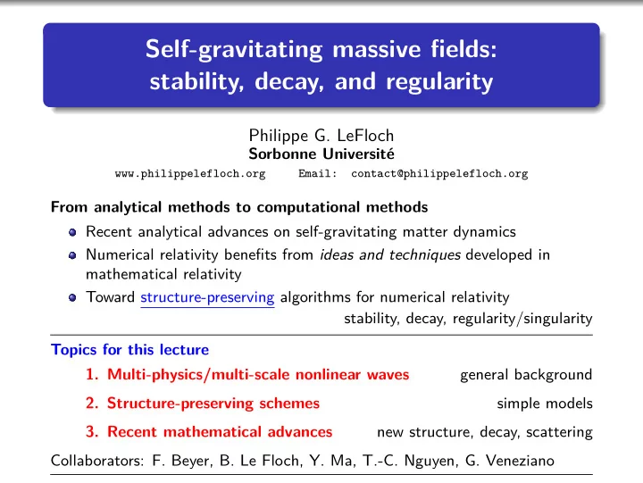
Self-gravitating massive fields: stability, decay, and regularity Philippe G. LeFloch Sorbonne Universit´ e www.philippelefloch.org Email: contact@philippelefloch.org From analytical methods to computational methods Recent analytical advances on self-gravitating matter dynamics Numerical relativity benefits from ideas and techniques developed in mathematical relativity Toward structure-preserving algorithms for numerical relativity stability, decay, regularity/singularity Topics for this lecture 1. Multi-physics/multi-scale nonlinear waves general background 2. Structure-preserving schemes simple models 3. Recent mathematical advances new structure, decay, scattering Collaborators: F. Beyer, B. Le Floch, Y. Ma, T.-C. Nguyen, G. Veneziano

1. Multi-physics and multi-scale nonlinear waves From first principles of continuum physics Massive fields and interfaces Klein-Gordon, complex fluids, modified gravity beyond Einstein gravity global dynamics of shocks, moving material interfaces, phase boundaries impulsive gravitational waves, cosmological singularities Fluids, gases, plasmas, solid materials liquid-vapor flows, thin liquid films, combustion waves, bores in shallow water, astrophysical flows, neutron stars, phase transformations Multi-scale wave phenomena many parameters viscosity, surface tension, heat, Hall effect, friction competitive effects several scales (fluid, geometry) fine-scale structure oscillations, turbulence Scale-sensitive nonlinear waves regime where one can extract variables with well-defined limits (despite possible oscillations) under-compressive shocks, subsonic liquid-gas boundaries, combustion waves, etc. “driving for” for the global dynamics

Diffusive-dispersive nonlinear wave propagation ∂ x ρ 3 = ε ∂ 2 ρ ∂ x 2 + κ ∂ 3 ρ ∂ t ρ + ∂ ∂ ∂ x 3 plane-symmetry, conservation law fluid density ρ = ρ ( t , x ) in a tube time t � 0 space x ∈ R viscosity ε << 1 surface tension/capillarity κ << 1 Intermolecular forces between a liquid and its surroundings Riemann problem single initial discontinuity, dam breaking problem

Three possible asymptotic regimes ε → 0 κ << ε 2 (viscosity is dominant) no oscillations, single limit κ = α ε 2 (balanced regime) mild oscillations, α -dependent limit κ >> ε 2 (surface tension is dominant, α fixed) oscillations, no limit Isothermal compressible fluids Van der Waals fluid two coupled conservation laws τ t − u x = 0 , u t + p ( v ) x = ε u xx − κ τ xxx 3 τ − 1 − 3 /τ 2 8 T specific volume τ velocity u pressure p ( τ ) = Typical Riemann wave structure 2.5 2.5 2.5 2.5 2.5 2.5 2.5 2.5 2.5 u L =0.2 0.8 3.5 2.25 2.25 2.25 2.25 2.25 2.25 2.25 2.25 2.25 0.75 u L =0.5 0.7 3 2 2 2 2 2 2 2 2 2 0.65 u L =.6 u L =0.7 0.6 1.75 1.75 1.75 1.75 1.75 1.75 1.75 1.75 1.75 2.5 0.55 u L =0.95 0.5 v v v v v v v v ! 1.5 1.5 1.5 1.5 1.5 1.5 1.5 1.5 1.5 u ! ! 0.45 2 u L =1.1 0.4 1.25 1.25 1.25 1.25 1.25 1.25 1.25 1.25 1.25 0.35 1.5 u L =1.3 0.3 1 1 1 1 1 1 1 1 1 0.25 u L =1.4 u L =1.5 1 0.75 0.75 0.75 0.75 0.75 0.75 0.75 0.75 0.75 0.2 0.15 0.5 0.5 0.5 0.5 0.5 0.5 0.5 0.5 0.5 0.1 0.2 0.3 0.4 0.5 0.6 0.7 0.2 0.3 0.4 0.5 0.6 0.7 0 0 0 0 0 0 0 0 0 0.25 0.25 0.25 0.25 0.25 0.25 0.25 0.25 0.25 0.5 0.5 0.5 0.5 0.5 0.5 0.5 0.5 0.5 0.75 0.75 0.75 0.75 0.75 0.75 0.75 0.75 0.75 1 1 1 1 1 1 1 1 1 x x x x x x x x x x x

Small-scale dependent nonlinear waves rules for connecting left- and right-hand state values from both sides beyond the standard Rankine-Hugoniot relations! notion of a kinetic function/scattering map for interfaces κ = α ε 2 varying the ratio surface tension/viscosity Structure-preserving algorithms front tracking • shock capturing with well-controled dissipation 2.5 2.5 2.5 2.5 2.5 2.5 2.5 2.5 2.5 u L =0.2 2.25 2.25 2.25 2.25 2.25 2.25 2.25 2.25 2.25 u L =0.5 2 2 2 2 2 2 2 2 2 u L =.6 u L =0.7 1.75 1.75 1.75 1.75 1.75 1.75 1.75 1.75 1.75 u L =0.95 1.5 1.5 1.5 1.5 1.5 1.5 1.5 1.5 1.5 ! v v v v v v v v ! u L =1.1 1.25 1.25 1.25 1.25 1.25 1.25 1.25 1.25 1.25 u L =1.3 1 1 1 1 1 1 1 1 1 u L =1.4 u L =1.5 0.75 0.75 0.75 0.75 0.75 0.75 0.75 0.75 0.75 0.5 0.5 0.5 0.5 0.5 0.5 0.5 0.5 0.5 0 0 0 0 0 0 0 0 0 0.25 0.25 0.25 0.25 0.25 0.25 0.25 0.25 0.25 0.5 0.5 0.5 0.5 0.5 0.5 0.5 0.5 0.5 0.75 0.75 0.75 0.75 0.75 0.75 0.75 0.75 0.75 1 1 1 1 1 1 1 1 1 x x x x x x x x x

2. Structure-preserving schemes: simple models Preserving the asymptotic structure on an inhomogeneous FLRW background joint with Y. Cao (Paris) and M. Ghazizadeh (Ottawa) ArXiv:1912.13439 Formulation of the problem 2 + 1 dim., isothermal, relativistic compressible flow p ( ρ ) = k 2 ρ FLRW-type cosmological background, with small inhomogeneities future-contracting geometry ( t < 0 and t → 0) ρ → + ∞ Asymptotic behavior toward the cosmological singularity nonlinear hyperbolic systems on a curved geometry ∂ t U + ∂ x F ( t , x , U ) = H ( t , x , U ) • two competitive effects contracting geometry shock propagation, nonlinear interactions • small-scale structure, driven by the (fixed) background geometry similar to phase transition dynamics (multiple scales)

Structure-preserving divergence form: finite volume scheme, shock-capturing (speed) high accuracy: 4th-order in time, 2nd-order in space, oscillation-free well-balanced property • introduce suitably rescaled unknowns (Fuchsian PDE method) • enforce the asymptotic state equations at the discrete level • enforce commutation property lim t → 0 lim ∆ x → 0 U = lim ∆ x → 0 lim t → 0 U Typical behavior: sharp transitions with spikes plots of the rescaled velocity component u and rescaled density � ρ 1.00 0.14 t = -1e-05 0.75 t = -1e-06 0.12 t = -1e-07 0.50 t = -1e-05 t = -1e-08 0.10 t = -1e-06 t = -1e-09 0.25 t = -1e-07 t = -1e-10 0.08 t = -1e-08 t = -1e-11 0.00 u t = -1e-09 t = -1e-12 t = -1e-10 0.06 0.25 t = -1e-11 t = -1e-12 0.04 0.50 0.02 0.75 1.00 0.00 0.0 0.2 0.4 0.6 0.8 1.0 0.0 0.2 0.4 0.6 0.8 1.0 x x

Times t = − 10 − 1 , − 10 − 3 , − 10 − 5 Standard algorithm Velocity magnitude V Rescaled density � ρ

Times t = − 10 − 1 , − 10 − 3 , − 10 − 5 Well-balanced algorithm Velocity magnitude V Rescaled density � ρ

Preserving the asymptotic structure on a Kasner background: evolution from the singularity joint with F. Beyer (Dunedin) ArXiv:2005.13504 Kasner geometry spatially homogeneous, anisotropic vacuum solution g = t ( K 2 − ) / 2 � − dt 2 + dx 2 + t 1 − K dy 2 + t 1+ K dz 2 M = (0 , + ∞ ) × T 3 with asymptotic velocity K ∈ R and Kasner exponents p 1 = K 2 − 1 p 2 = 2(1 − K ) p 3 = 2(1 + K ) K 2 + 3 , K 2 + 3 , K 2 + 3 Compressible fluid flow with pressure law p = ( γ − 1) ρ with γ ∈ (1 , 2) Characteristic exponent � 3 γ − 2 − K 2 (2 − γ ) � Γ = 1 ∈ (0 , 1) 4 which compare the geometry and fluid behaviors Γ > 0 : sub-critical regime dynamically stable Γ � 0 : super-critical / critical regimes dynamically unstable Formally, plug an expansion in power of t and attempt to validate it (Fuchsian asymptotics)

Evolution from the cosmological singularity t = 0 formulate a singular initial value problem B 0 ( U , t , x ) ∂ t U + B 1 ( U , t , x ) ∂ x U = f ( U , t , x ) suitable “singular initial data” prescribed on t = 0 Fuchsian-type expansions near the cosmological singularity sufficiently regular, shock-free regime Algorithm preserving the Fuchsian structure discretize U ( t , x ) ≃ V ( t ) = ( V j ( t )) by the pseudo-spectral method of lines ∂ t V − AV = h ( V , t ) high-order Runge-Kutta discretization in time introduce suitably rescaled variables rigorous analysis of the numerical error: take into account the Fuchsian expansion two sources of approximation error: continuum / discrete our proposal : keep the two error sources asymptotically in balance With this numerical strategy, we numerically demonstrated the nonlinear stability of the flow near the cosmological singularity the sub-critical regime.

Numerical results for a typical evolution from the singularity – fluid density (contour plot) and velocity field (flow lines) – time (vertically) the density ρ is unbounded in the limit t → 0 we carefully checked the numerical error reliable algorithm, despite the solutions being very singular 1 . 2 1 . 2 1 10 − 2 0 − 2 − 2 0 1 0 0 0 − 1 1 . 0 1 . 0 1 1 10 − 1 0 . 8 0 . 8 10 1 10 0 0 . 6 0 . 6 t t 1 1 0 0 . 4 0 . 4 0 2 1 0 . 2 0 . 2 10 3 1 0 4 0 . 0 0 . 0 0 . 0 0 . 5 1 . 0 1 . 5 0 . 0 0 . 5 1 . 0 1 . 5 2 . 0 x/π x/π

Numerical results: evolution V ε toward the singularity by adding a perturbation ε on the data at time t = T > 0 regime far from linear perturbation theory compute the perturbed singular data V ε 0 reached on t = 0 compare to the given unperturbed data V 0 0 → V ε as ε → 0 stability/continuous dependence: V ε 250 200 | V ǫ, ∞ − V ∗ | 150 100 50 0 0 . 0000 0 . 0005 0 . 0010 0 . 0015 0 . 0020 0 . 0025 0 . 0030 ǫ Extension to self-gravitating fluids: in progress