Segmentation methods It makes a hard decision too soon. We want to - - PDF document

SLIDE 1

1 Segmentation and low-level grouping.

Bill Freeman, MIT 6.869 April 14, 2005 Readings: Mean shift paper and background segmentation paper.

• Mean shift IEEE PAMI paper by Comanici and

Meer,

http://www.caip.rutgers.edu/~comanici/Papers/MsRobustApproach.pdf

• Forsyth&Ponce, Ch. 14, 15.1, 15.2.
• Wallflower: Principles and Practice of

Background Maintenance, by Kentaro Toyama, John Krumm, Barry Brumitt, Brian Meyers.

http://research.microsoft.com/users/jckrumm/Publications%202000/Wall%20Flower.pdf

The generic, unavoidable problem with low-level segmentation and grouping

• It makes a hard decision too soon. We want to

think that simple low-level processing can identify high-level object boundaries, but any implementation reveals special cases where the low-level information is ambiguous.

• So we should learn the low-level grouping

algorithms, but maintain ambiguity and pass along a selection of candidate groupings to higher processing levels.

Segmentation methods

• Segment foreground from background
• K-means clustering
• Mean-shift segmentation
• Normalized cuts

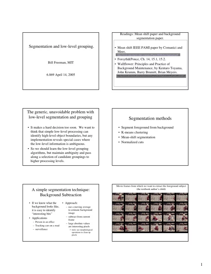
A simple segmentation technique: Background Subtraction

• If we know what the

background looks like, it is easy to identify “interesting bits”

• Applications

– Person in an office – Tracking cars on a road – surveillance

• Approach:

– use a moving average to estimate background image – subtract from current frame – large absolute values are interesting pixels

• trick: use morphological
• perations to clean up

pixels

Movie frames from which we want to extract the foreground subject (the textbook author’s child)

SLIDE 2

2

low thresh high thresh EM

2 different background removal models

Background estimate Foreground estimate Foreground estimate

Average over frames EM background estimate

Static Background Modeling Examples

[MIT Media Lab Pfinder / ALIVE System]

Static Background Modeling Examples

[MIT Media Lab Pfinder / ALIVE System]

Static Background Modeling Examples

[MIT Media Lab Pfinder / ALIVE System]

BG Pixel distribution is non-stationary:

Dynamic Background

[MIT AI Lab VSAM]

Staufer and Grimson tracker: Fit per-pixel mixture model to observed distrubution.

Mixture of Gaussian BG model

[MIT AI Lab VSAM]

SLIDE 3

3

http://research.microsoft.com/users/toyama/wallflower.pd

Background removal issues

http://research.microsoft.com/users/toyama/wallflower.pd

Background Subtraction Principles

Wallflower: Principles and Practice of Background Maintenance, by Kentaro Toyama, John Krumm, Barry Brumitt, Brian Meyers. P1: P2: P3: P4: P5:

Background Techniques Compared

From the Wallflower Paper

Segmentation as clustering

• Cluster together (pixels, tokens, etc.) that belong

together…

• Agglomerative clustering

– attach closest to cluster it is closest to – repeat

• Divisive clustering

– split cluster along best boundary – repeat

• Dendrograms

– yield a picture of output as clustering process continues

Greedy Clustering Algorithms

SLIDE 4

4

Data set Dendrogram formed by agglomerative clustering using single-link clustering.

Segmentation methods

• Segment foreground from background
• K-means clustering
• Mean-shift segmentation
• Normalized cuts

K-Means

• Choose a fixed number of

clusters

• Choose cluster centers and

point-cluster allocations to minimize error

• can’t do this by search,

because there are too many possible allocations.

• Algorithm

– fix cluster centers; allocate points to closest cluster – fix allocation; compute best cluster centers

• x could be any set of

features for which we can compute a distance (careful about scaling) x j − µi

2 j∈elements of i'th cluster

∑

⎧ ⎨ ⎩ ⎫ ⎬ ⎭

i∈clusters

∑

K-Means

Matlab k-means clustering demo

K-means clustering using intensity alone and color alone

Image Clusters on intensity (K=5) Clusters on color (K=5)

SLIDE 5

5

K-means using color alone, 11 segments

Image Clusters on color

K-means using color alone, 11 segments.

Color alone

• ften will not

yeild salient segments!

Ways to include spatial relationships

(a) Define a Markov Random Field (MRF), where the state to be estimated includes the segment index. Solve by graph cuts or BP. (b) Augment data to be clustered with spatial coordinates.

⎟ ⎟ ⎟ ⎟ ⎟ ⎟ ⎠ ⎞ ⎜ ⎜ ⎜ ⎜ ⎜ ⎜ ⎝ ⎛ = y x v u Y z

color coordinates spatial coordinates K-means using colour and position, 20 segments

Still misses goal of perceptually pleasing segmentation! Hard to pick K…

Segmentation methods

• Segment foreground from background
• K-means clustering
• Mean-shift segmentation
• Normalized cuts

Mean Shift Segmentation

http://www.caip.rutgers.edu/~comanici/MSPAMI/msPamiResults.html

SLIDE 6

6

Mean Shift Algorithm

Mean Shift Algorithm

• 1. Choose a search window size.
• 2. Choose the initial location of the search window.
• 3. Compute the mean location (centroid of the data) in the search window.
• 4. Center the search window at the mean location computed in Step 3.
• 5. Repeat Steps 3 and 4 until convergence.

The mean shift algorithm seeks the “mode” or point of highest density of a data distribution:

Mean Shift Segmentation Algorithm

• 1. Convert the image into tokens (via color, gradients, texture measures etc).
• 2. Choose initial search window locations uniformly in the data.
• 3. Compute the mean shift window location for each initial position.
• 4. Merge windows that end up on the same “peak” or mode.
• 5. The data these merged windows traversed are clustered together.

*Image From: Dorin Comaniciu and Peter Meer, Distribution Free Decomposition of Multivariate Data, Pattern Analysis & Applications (1999)2:22–30

Mean Shift Segmentation

• For your homework, you will do a mean

shift algorithm just in the color domain. In the slides that follow, however, both spatial and color information are used in a mean shift segmentation.

Comaniciu and Meer, IEEE PAMI vol. 24, no. 5, 2002

Apply mean shift jointly in the image (left col.) and range (right col.) domains

5 1 7 1

Window in image domain

0 1 3

Window in range domain

0 1 2

Intensities of pixels within image domain window

4

Center of mass of pixels within both image and range domain windows

0 1 6

Center of mass of pixels within both image and range domain windows

Mean Shift color&spatial Segmentation Results:

http://www.caip.rutgers.edu/~comanici/MSPAMI/msPamiResults.html

SLIDE 7

7

Mean Shift color&spatial Segmentation Results:

Segmentation methods

• Segment foreground from background
• K-means clustering
• Mean-shift segmentation
• Normalized cuts

Graph-Theoretic Image Segmentation

Build a weighted graph G=(V,E) from image V:image pixels E: connections between pairs of nearby pixels region same the to belong j & i y that probabilit :

ij

W

Graphs Representations

a e d c b ⎥ ⎥ ⎥ ⎥ ⎥ ⎥ ⎦ ⎤ ⎢ ⎢ ⎢ ⎢ ⎢ ⎢ ⎣ ⎡ 1 1 1 1 1 1 1 1 Adjacency Matrix

* From Khurram Hassan-Shafique CAP5415 Computer Vision 2003

Weighted Graphs and Their Representations

a e d c b ⎥ ⎥ ⎥ ⎥ ⎥ ⎥ ⎦ ⎤ ⎢ ⎢ ⎢ ⎢ ⎢ ⎢ ⎣ ⎡ ∞ ∞ ∞ ∞ ∞ ∞ 1 7 2 1 6 7 6 4 3 2 4 1 3 1 Weight Matrix 6

* From Khurram Hassan-Shafique CAP5415 Computer Vision 2003

Boundaries of image regions defined by a number of attributes

– Brightness/color – Texture – Motion – Stereoscopic depth – Familiar configuration [Malik]

SLIDE 8

8

Measuring Affinity

Intensity Color Distance aff x, y

( )= exp −

1 2σ i

2

⎛ ⎝ ⎞ ⎠ I x

( )− I y ( )

2

( )

⎧ ⎨ ⎩ ⎫ ⎬ ⎭ aff x, y

( )= exp −

1 2σ d

2

⎛ ⎝ ⎞ ⎠ x − y

2

( )

⎧ ⎨ ⎩ ⎫ ⎬ ⎭ aff x, y

( )= exp −

1 2σ t

2

⎛ ⎝ ⎞ ⎠ c x

( )− c y ( )

2

( )

⎧ ⎨ ⎩ ⎫ ⎬ ⎭

Eigenvectors and affinity clusters

• Simplest idea: we want a

vector a giving the association between each element and a cluster

• We want elements within

this cluster to, on the whole, have strong affinity with one another

• We could maximize
• But need the constraint
• This is an eigenvalue

problem (p. 321 of Forsyth&Ponce)

• choose the

eigenvector of A with largest eigenvalue

aTAa aTa = 1

Example eigenvector

points matrix eigenvector

Example eigenvector

points matrix eigenvector

Scale affects affinity

σ=.2 σ=.1 σ=.2 σ=1

Some Terminology for Graph Partitioning

• How do we bipartition a graph:

∅ = ∩ ∈ ∈∑

=

B A with B A,

), , W( B) A, (

v u

v u cut

disjoint y necessaril not A' and A A' A,

) , ( W ) A' A, (

∑

∈ ∈

=

v u

v u assoc

[Malik]

SLIDE 9

9

Minimum Cut

A cut of a graph G is the set of edges S such that removal of S from G disconnects G. Minimum cut is the cut of minimum weight, where weight of cut <A,B> is given as

( )

( )

∑

∈ ∈

=

B y A x

y x w B A w

,

, ,

* From Khurram Hassan-Shafique CAP5415 Computer Vision 2003

Minimum Cut and Clustering

* From Khurram Hassan-Shafique CAP5415 Computer Vision 2003

Drawbacks of Minimum Cut

• Weight of cut is directly proportional to the

number of edges in the cut.

Ideal Cut Cuts with lesser weight than the ideal cut

* Slide from Khurram Hassan-Shafique CAP5415 Computer Vision 2003

Normalized cuts

• First eigenvector of affinity

matrix captures within cluster similarity, but not across cluster difference

• Min-cut can find degenerate

clusters

• Instead, we’d like to maximize

the within cluster similarity compared to the across cluster difference

• Write graph as V, one cluster as

A and the other as B

• Minimize

where cut(A,B) is sum of weights with one end in A and one end in B; assoc(A,V) is sum of all edges with one end in A. I.e. construct A, B such that their within cluster similarity is high compared to their association with the rest of the graph

cut(A,B) assoc(A,V) cut(A,B) assoc(B,V) +

Solving the Normalized Cut problem

• Exact discrete solution to Ncut is NP-complete

even on regular grid,

– [Papadimitriou’97]

• Drawing on spectral graph theory, good

approximation can be obtained by solving a generalized eigenvalue problem.

[Malik]

Normalized Cut As Generalized Eigenvalue problem

after simplification, Shi and Malik derive ... ) , ( ) , ( ; 1 1 ) 1 ( ) 1 )( ( ) 1 ( 1 1 ) 1 )( ( ) 1 ( ) V B, ( ) B A, ( ) V A, ( B) A, ( B) A, ( = = − − − − + + − + = + =

∑ ∑ >

i x T T T T

i i D i i D k D k x W D x D k x W D x assoc cut assoc cut Ncut

i

. 1 }, , 1 { with , ) ( ) , ( = − ∈ − = D y b y Dy y y W D y B A Ncut

T i T T

[Malik]

∑

=

j ij ii

A D

SLIDE 10

10 Normalized cuts

• Instead, solve the generalized eigenvalue problem
• which gives
• They show that the 2nd smallest eigenvector solution y is a good real-

valued appox to the original normalized cuts problem. Then you look for a quantization threshold that maximizes the criterion --- i.e all components of y above that threshold go to one, all below go to -b

maxy yT D − W

( )y

( ) subject to yTDy = 1 ( )

D − W

( )y = λDy

http://www.cs.berkeley.edu/~malik/papers/SM-ncut.pdf

Brightness Image Segmentation

http://www.cs.berkeley.edu/~malik/papers/SM-ncut.pdf

Brightness Image Segmentation

http://www.cs.berkeley.edu/~malik/papers/SM-ncut.pdf http://www.cs.berkeley.edu/~malik/papers/SM-ncut.pdf

Results on color segmentation

http://www.cs.berkeley.edu/~malik/papers/SM-ncut.pdf

Nice web page on grouping from Malik’s group.

SLIDE 11

11

Contains a large dataset of images with human “ground truth” labeling. Of course, the human labelings differ one from another.

• Hough transform
• Iterative fitting

Line Fitting Fitting

• Choose a parametric
• bject/some objects to

represent a set of tokens

• Most interesting case is

when criterion is not local

– can’t tell whether a set of points lies on a line by looking only at each point and the next.

• Three main questions:

– what object represents this set of tokens best? – which of several objects gets which token? – how many objects are there? (you could read line for object here, or circle, or ellipse

• r...)

Fitting and the Hough Transform

• Purports to answer all three

questions

– in practice, answer isn’t usually all that much help

• We do for lines only
• A line is the set of points (x, y)

such that

• Different choices of θ, d>0 give

different lines

• For any (x, y) there is a one

parameter family of lines through this point, given by

• Each point gets to vote for each

line in the family; if there is a line that has lots of votes, that should be the line passing through the points

sinθ

( )x + cosθ ( )y + d = 0

sinθ

( )x + cosθ ( )y + d = 0

tokens

θ d

Votes for parameter values satisfying at each token sinθ

( )x + cosθ ( )y + d = 0

SLIDE 12

12 Mechanics of the Hough transform

• Construct an array

representing θ, d

• For each point, render the

curve (θ, d) into this array, adding one at each cell

• Difficulties

– how big should the cells be? (too big, and we cannot distinguish between quite different lines; too small, and noise causes lines to be missed)

• How many lines?

– count the peaks in the Hough array

• Who belongs to which

line?

– tag the votes

• Problems with noise and

cell size can defeat it

tokens votes

Rules of thumb for getting Hough transform to work well

• Can work for finding lines in a set of edge

points.

• Ensure minimum number of irrelevant

tokens by tuning the edge detector.

• Choose the quantization grid carefully by

trial and error.

SLIDE 13

13

What criteria to optimize when fitting a line to a set of points?

Line fitting

Line fitting can be max. likelihood - but choice of model is important “Total Least Squares” “Least Squares”

Who came from which line?

• Assume we know how many lines there are
• but which lines are they?

– easy, if we know who came from which line

• Three strategies

– Incremental line fitting – K-means (described in book) – Probabilistic (in book, and in earlier lecture notes)

Incremental line fitting Incremental line fitting

SLIDE 14

14

Incremental line fitting Incremental line fitting Incremental line fitting Fitting contours

• Two common techniques:

– Snakes (Terzopolous, Witkin, and Kass) – Dynamic programming methods

http://www.cs.huji.ac.il/~shashua/papers/saliency.pdf

http://people.csail.mit.edu/people/billf/freemanThesis.pdf

SLIDE 15

15

http://people.csail.mit.edu/people/billf/freemanThesis.pdf http://people.csail.mit.edu/people/billf/freemanThesis.pdf

http://www.cs.huji.ac.il/~shashua/papers/saliency.pdf