
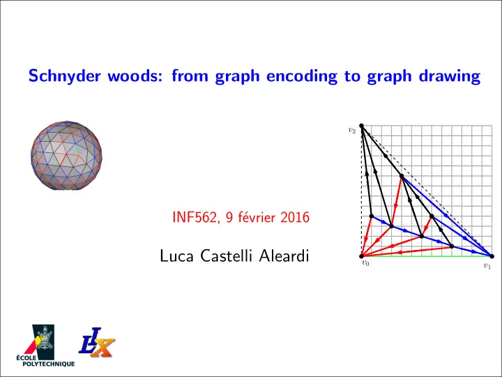
SLIDE 1
Luca Castelli Aleardi
INF562, 9 f´ evrier 2016
v0 v1 v2
Schnyder woods: from graph encoding to graph drawing
Schnyder woods: from graph encoding to graph drawing v 2 INF562, 9 f - - PowerPoint PPT Presentation
Schnyder woods: from graph encoding to graph drawing v 2 INF562, 9 f evrier 2016 Luca Castelli Aleardi v 0 v 1 Some facts about planar graphs (As I have known them) Some facts about planar graphs Thm (Schnyder, Trotter, Felsner) G
Luca Castelli Aleardi
INF562, 9 f´ evrier 2016
v0 v1 v2
Schnyder woods: from graph encoding to graph drawing
(”As I have known them”)
G planar if and only if G contains neither K5 nor K3,3 as minors Thm (Schnyder, Trotter, Felsner) Every planar graph with n vertices is isomorphic to the intersection graph of n disks in the plane. Thm (Koebe-Andreev-Thurston)
Thm (Kuratowski, excluded minors) G planar if and only if dim(G) ≤ 3 Thm (Y. Colin de Verdi` ere) G planar if and only if µ(G) ≤ 3 (µ(G) = multiplicity of λ2 of a generalized laplacian) vN S2 vN M 4 −1 . . . −1 5 . . . 3 LG = . . . . . . . . . . . . . . . . . .
LG[i, k] = { −AG[i, j] deg(vi)
Every planar graph with n vertices is isomorphic to the intersection graph of n disks in the plane. Thm (Koebe-Andreev-Thurston)
(images by N. Bonichon)
Every planar graph with n vertices is isomorphic to the intersection graph of n disks in the plane. Thm (Koebe-Andreev-Thurston)
(images by N. Bonichon) (images by R. Silveira) Not every planar triangulation is Delaunay realizable
TD-Delaunay: triangular distance Delaunay triangulations Thm (de Fraysseix, Ossona de Mendez, Rosenstiehl, ’94)
(images by S. Felsner)
Chew, ’89
(images by N. Bonichon)
Every planar triangulation is TD-Delaunay realizable
1 2 3 4 5 10 8 12 21 19 24 15 22 17 23 18 16 7 13 9 11 20 6 14
φ = (1, 2, 3, 4)(17, 23, 18, 22)(5, 10, 8, 12)(21, 19, 24, 15) . . . α = (2, 18)(4, 7)(12, 13)(9, 15)(14, 16)(10, 23) . . .
n − e + f = 2 e = 3n − 6
S2
Schnyder woods and canonical orderings: overview of applications
(graph drawing, graph encoding, succinct representations, compact data structures, exhaustive graph enumeration, bijective counting, greedy drawings, spanners, contact representations, planarity testing, untangling of planar graphs, Steinitz representations of polyhedra, . . .)
bijective counting, random generation
1 2 3 4 5 6 7 8 9 10 11 4 3 2 5 6 7 8 9 10 1 1 2 3 4 5 6 7 8 9
) ( ( ( ( ( ) ) ( ) ( ) ) ( ) ( ( ) ) ( ) ( ) ) [ ] [ [ [ ] ] ] [ [ ] ]
[ [ [ [
] ] ]
]
{ } { } { { } { } { { { } } } { } } S
T0 T1 T2
(Poulalhon-Schaeffer, Icalp 03)
Graph encoding
Thm (Schnyder ’90) planar straight-line grid drawing (on a O(n × n) grid)
cn =
2(4n+1)! (3n+2)!(n+1)!
⇒ optimal encoding ≈ 3.24 bits/vertex (Chuang, Garg, He, Kao, Lu, Icalp’98) (He, Kao, Lu, 1999)
u v a b
Every planar triangulation admits a greedy drawing (Dhandapani, Soda08) (conjectured by Papadimitriou and Ratajczak for 3-connected planar graphs)
Greedy routing
Schnyder woods, TD-Delaunay graphs, orthogonal surfaces and Half-Θ6-graphs
[ Bonichon et al., WG’10, Icalp ’10, ...]
(the definition)
v0 v1 n nodes v2
ii) colors and orientations around each inner node must respect the local Schnyder condition
i) edge are colored and oriented in such a way that each inner nodes has exaclty one outgoing edge of each color
A Schnyder wood of a (rooted) planar triangulation is partition of all inner edges into three sets T0, T1 and T2 such that
[Schnyder ’90] rooted triangulation on
v0 v1 v2 [3-orientation] [normal labeling]
0 0 2 2 2 2 2 2 2 2 2 1 1 1 1 1 1 1 1 1 1 1 1 1 2 2 2 2
1 1 2 3-connected graphs [Felsner]
1 2
v0 v1 v2 [Schnyder ’90]
Theorem The three sets T0, T1, T2 are spanning trees of the inner vertices of T (each rooted at vertex vi)
v1 v0
T2 T1
v2
T0
v0 v1 [incremental vertex shelling, Brehm’s thesis]
Theorem Every planar triangulation admits a Schnyder wood, which can be computed in linear time.
The traversal starts from the root face
v0 v1 [incremental vertex shelling, Brehm’s thesis]
Theorem Every planar triangulation admits a Schnyder wood, which can be computed in linear time.
The traversal starts from the root face
vn−1 ⇓
Gk−1 Gk
perform a vertex conquest at each step
vk
v0 v1 [incremental vertex shelling, Brehm’s thesis]
Theorem Every planar triangulation admits a Schnyder wood, which can be computed in linear time.
The traversal starts from the root face
vn−2 w ⇓
Gk−1 Gk
perform a vertex conquest at each step
vk
v0 v1 [incremental vertex shelling, Brehm’s thesis]
Theorem Every planar triangulation admits a Schnyder wood, which can be computed in linear time.
The traversal starts from the root face
vn−3 ⇓
Gk−1 Gk
perform a vertex conquest at each step
vk
v0 v1 [incremental vertex shelling, Brehm’s thesis]
Theorem Every planar triangulation admits a Schnyder wood, which can be computed in linear time.
The traversal starts from the root face
⇓
Gk−1 Gk
perform a vertex conquest at each step
vk
v0 v1 [incremental vertex shelling, Brehm’s thesis]
Theorem Every planar triangulation admits a Schnyder wood, which can be computed in linear time.
The traversal starts from the root face
Invariant:
vk u
v0 v1 [incremental vertex shelling, Brehm’s thesis]
Theorem Every planar triangulation admits a Schnyder wood, which can be computed in linear time.
The traversal starts from the root face
Invariant:
vk u
v0 v1 [incremental vertex shelling, Brehm’s thesis]
Theorem Every planar triangulation admits a Schnyder wood, which can be computed in linear time.
The traversal starts from the root face
Invariant:
vk u
v0 v1 [incremental vertex shelling, Brehm’s thesis]
Theorem Every planar triangulation admits a Schnyder wood, which can be computed in linear time.
The traversal starts from the root face
v2
Invariant:
vk u
(the definition)
[de Fraysseix Pach Pollack]
e
1
G1 = {0, 1, 2}
e
2
e
3
G3 G2
e
4
G4
e
5
G5
G = G7
6 7 8
(of planar graphs)
[Wagner’36] [Fary’48]
⇒
[Wagner’36] [Fary’48]
⇒
Classical algorithms:
[Tutte’63] [De Fraysseix, Pach, Pollack 89] [Schnyder’90] spring-embedding incremental (Shift-algorithm) face-counting principle
existence of straight-line drawing
[Stein’51]
[Wagner’36] [Fary’48]
⇒
[Wagner’36] [Fary’48]
⇒
A B C D E G Output geometric coordinates of vertices F Input of the problem set of triangle faces a b c d e f g h i (a, b, c) (a, c, d) (d, c, e) (c, b, e) (a, d, f) (f, d, g) (d, e, g) (e, b, g) (a, f, h) (a, h, i) (i, h, f) (i, f, g) (i, g, b) (i, b, a)
Barycentric representation of a planar graph
Barycentric representation of a planar graph
c b a v2 v v1 v0
v = v0a + v1b + v2c where vi is the normalized area
Barycentric representation def:
f(v) − → (v0, v1, v2) ∈ R3 v0 + v1 + v2 = 1 , for each vertex v for each edge (x, y) ∈ E and each vertex z / ∈ {x, y} there is an index k ∈ {0, 1, 2} such that xk < zk yk < zk
Barycentric representation of a planar graph
Barycentric representation def:
f(v) − → (v0, v1, v2) ∈ R3 v0 + v1 + v2 = 1 , for each vertex v
(1, 0, 0) (0, 1, 0) (0, 0, 1)
a b c
Barycentric representation of a planar graph
Barycentric representation def:
f(v) − → (v0, v1, v2) ∈ R3 v0 + v1 + v2 = 1 , for each vertex v for each edge (x, y) ∈ E and each vertex z / ∈ {x, y} there is an index k ∈ {0, 1, 2} such that xk < zk yk < zk
(1, 0, 0) (0, 1, 0) (0, 0, 1) (1, 0, 0) (0, 1, 0) (0, 0, 1) f(x) f(y) f(z)
no vertex z in the gray triangle defined by f(x), f(y)
max(x2, y2) max(x0, y0)
Barycentric representation of a planar graph
Theorem A barycentric representation defines a planar straight-line drawing of G, in the plane spanned by (1, 0, 0), (0, 1, 0) and (0, 0, 1).
for each edge (x, y) ∈ E and each vertex z / ∈ {x, y}, f(z) cannot lie on (f(x), f(y))
(1, 0, 0) (0, 1, 0) (0, 0, 1) f(x) f(y) f(z) max(x2, y2) max(x0, y0)
f(z) = tf(x) + (1 − t)f(y) , for t ∈ [0, 1] zk = txk + (1 − t)yk) < tzk + (1 − t)zk = zk for k ∈ {0, 1, 2}
Barycentric representation of a planar graph
Theorem A barycentric representation defines a planar straight-line drawing of G, in the plane spanned by (1, 0, 0), (0, 1, 0) and (0, 0, 1).
given two edges (x, y), (u, v) ∈ E they cannot cross
f(x) f(y) f(u)
ui, vi < xi
f(v)
by definition there are four indices i, j, k, l ∈ {0, 1, 2} uj, vj < yj xk, yk < uk xl, yl < vl i = k, l and j = k, l i = j or k = l assume i = j = 2 there exists a separating line l parallel to [(1, 0, 0), (0, 1, 0)]
l
if i = k we would have uk < xk vk < xk contradicting xk, yk < uk
(Schnyder algorithm, 1990)
x1 x3 x2 R1(v) v R3(v) R2(v)
v = |R1(v)|
|T |
x1 + |R2(v)|
|T |
x2 + |R3(v)|
|T |
x3 where |Ri(v)| is the number of triangles
Theorem (Schnyder, Soda ’90) For a triangulation T having n vertices, we can draw it on a grid of size (2n − 5) × (2n − 5), by setting x1 = (2n − 5, 0), x2 = (0, 0) and x3 = (0, 2n − 5).
x1 x3 x2 α1 v α3 α2
v = α1x1 + α2x2 + α3x3 where αi is the normalized area
Geometric interpretation
c b a R2(v) v R1(v) R0(v) c b a v
c b a
Ri(v)
v u c b a
Ri(u)
v u
if u ∈ Ri(v) Ri(u) ⊂ Ri(v) ui < vi
c b a
Ri(v)
v u c b a v
Pi+1(v) Pi−1(v) how to efficiently compute |Ri(v)|? t1 t2 t3 t4
⇒
T endowed with a Schnyder wood Input: T
a b c d e f g h i d a b c d e f g h i
→ (0, 0) → (0, 1) → (1, 0) → ( 5
13, 6 13)
→ ( 9
13, 1 13)
→ ( 7
13, 4 13)
→ ( 3
13, 3 13)
→ ( 4
13, 8 13)
→ ( 1
13, 4 13)
⇒
T endowed with a Schnyder wood Input: T
a b c d e f g h i d a b c d e f g h i
→ (13, 0, 0) → (0, 13, 0) → (0, 0, 13) → ( → (9, 3, 1) → (2, 7, 4) → (7, 3, 3) → (1, 4, 8) → (8, 1, 4)
d
5, 6, 2 )
⇒
T endowed with a Schnyder wood Input: T
a b c d e f g h i a b c d e f g h i
→ (13, 0, 0) → (0, 13, 0) → (0, 0, 13) → ( → (9, 3, 1) → (2, 7, 4) → (7, 3, 3) → (1, 4, 8) → (8, 1, 4)
d
5, 6, 2 )
⇒
T endowed with a Schnyder wood Input: T
a b c d e f g h i a b c d e f g h i
→ (13, 0, 0) → (0, 13, 0) → (0, 0, 13) → ( → (9, 3, 1) → (2, 7, 4) → (7, 3, 3) → (1, 4, 8) → (8, 1, 4)
d
5, 6, 2 )
Geometric v.s combinatorial information
Geometry between 30 et 96 bits/vertex vertex triangle 1 reference to a triangle 3 references to vertices 3 references to triangles ”Connectivity”: the underlying triangulation
13n log n 416n bits
vertex coordinates adjacency relations between triangles, vertices
#{triangulations} =
2(4n + 1)! (3n + 2)!(n + 1)! ≈ 16 27
2πn−5/2 256 27 n
⇒ entropy = log2
256 27 ≈ 3.24 bpv.
David statue (Stanford’s Digital Michelangelo Project, 2000) 2 billions polygons
32 Giga bytes (without compression)
No existing algorithm nor data structure for dealing with the entire model
( ) ( ( ( ) ) ( ) ( ) ) ( ) ( ( ) ) ( ) ( )
2 3 4 5 6 7 8 9 10 11
[[[[ ] ] ][[[ [ ]][ ]][[[[[ [ ]][ ]] ][ [ ]]][ ]]]] G \ T
T T
([[[)(](][[[)])(]][) . . . S(G)
Turan encoding of planar map (1984) length(S) = 2e symbols (2 log2 4)e = 4e = 12n bits G = (V, E) |V | = n |E| = e
T := (any) vertex spanning tree of G
parenthesis word of size 2n
12n bits encoding scheme
parenthesis word of size 2n
1
Canonical orderings - Schnyder woods (He, Kao, Lu ’99) 2 3 4 5 6 7 8 9 10 11 T0 T1 T2
Canonical orderings - Schnyder woods (He, Kao, Lu ’99) 2 3 4 5 6 7 8 9 10 11
T1 T2
T 0
1
Canonical orderings - Schnyder woods (He, Kao, Lu ’99) 2 3 4 5 6 7 8 9 10 11
T2
T1 is redundant: reconstruct from T0, T2
1 1
T 0
Canonical orderings - Schnyder woods (He, Kao, Lu ’99) 2 3 4 5 6 7 8 9 10 11
T2
T1 is redundant: reconstruct from T0, T2
1 1
T2 can be reconstructed from T0 and the number of ingoing edges (for each node)
2 3 4 5 6 7 8 9 10 11
T2
1 1
T 0 T 0
2 3 4 5 6 7 8 9 10 11
T2
1 1 2 3 4 5 6 7 8 9 10 11
T2
1 1
( ) ( ( ( ) ) ( ) ( ) ) ( ) ( ( ) ) ( ) ( )
T 0 T 0 T 0
2(n − 1) symbols= 2(n − 1) bits
00000101010100110111 T 2
(n − 1) + (n − 3) = 2n − 4 bits Canonical orderings - Schnyder woods (He, Kao, Lu ’99)
4n bits (for triangulations)
u v w z u v w z 1 2 3 u v w z u v w z
u := source(e) = e/3 (w,v):=T[2e] e := (u, v)
T[T[e]] (T[e] + 2)%3 u v w
Def.
z (z, v) := T[2e + 1] 0 ≤ v ≤ n − 1 0 ≤ e ≤ 3n
First simple Compact DS (size 6n)
case 1 case 2 case 3 (w, u) := color(e) = e%3 retrieve retrieving (z, u) is similar
implementation:
case analysis for black edges
More compact DS (size 5n): use minimal Schnyder woods
(less redundant and ”slightly more difficult to implement”)
many cases to distinguish
T[T[T[5u]]] case 1a case 1b . . . (w, u) := retrieve . . .
Half-edge Triangle-based
(non compact) data structures compact data structures
e
prev(e) next(e) source(e) Winged-edge Data Structure size navigation time vertex access dynamic Half-edge/Winged-edge/Quad-edge Triangle based DS / Corner Table Directed edge (Campagna et al. ’99) 2D Catalogs (Castelli Aleardi et al., ’06) Star vertices (Kallmann et al. ’02) TRIPOD (Snoeyink, Speckmann, ’99) SOT (Gurung et al. 2010) Castelli Aleardi and Devillers (2011)
18n + n 12n + n 12n + n 7.67n 7n 6n 6n 4.8n 4n
(or 6n) O(1) O(1) O(1) O(1) O(1) O(1) O(1) O(1) O(1) O(1) O(1) O(1) O(1) O(d) O(d) O(d) O(d) O(d) yes yes yes yes no no no yes no SQUAD (Gurung et al. 2011)
(4 + ε)n
O(1) O(d) no LR (Gurung et al. 2011)
(2 + δ)n
O(1) O(d) no ε between 0.09 and 0.3 δ about 0.8 and 0.3 ESQ (Castelli Aleardi, Devillers, Rossignac’12) (or O(1))
Compact (practical) mesh data structures
Half-edge, Winged-edge, Quad-edge (19n) Triangle DS, Corner Table, Directed edge (13n) 2D Catalogs (7.67n) (7n) Star-Vertices SOT (6n) Castelli Devillers (Isaac 2011), (4n) ESQ, (4.8n)
Half-edge Triangle-based
(non compact) data structures compact data structures
e
prev(e) next(e) source(e) Winged-edge Data Structure size navigation time vertex access dynamic Half-edge/Winged-edge/Quad-edge Triangle based DS / Corner Table Directed edge (Campagna et al. ’99) 2D Catalogs (Castelli Aleardi et al., ’06) Star vertices (Kallmann et al. ’02) TRIPOD (Snoeyink, Speckmann, ’99) SOT (Gurung et al. 2010) Castelli Aleardi and Devillers (2011)
18n + n 12n + n 12n + n 7.67n 7n 6n 6n 4.8n 4n
(or 6n) O(1) O(1) O(1) O(1) O(1) O(1) O(1) O(1) O(1) O(1) O(1) O(1) O(1) O(d) O(d) O(d) O(d) O(d) yes yes yes yes no no no yes no SQUAD (Gurung et al. 2011)
(4 + ε)n
O(1) O(d) no LR (Gurung et al. 2011)
(2 + δ)n
O(1) O(d) no ε between 0.09 and 0.3 δ about 0.8 and 0.3 ESQ (Castelli Aleardi, Devillers, Rossignac’12) (or O(1))
Compact (practical) mesh data structures
Half-edge, Winged-edge, Quad-edge (19n) Triangle DS, Corner Table, Directed edge (13n) 2D Catalogs (7.67n) (7n) Star-Vertices SOT (6n) Castelli Devillers (Isaac 2011), (4n) ESQ, (4.8n) vertex degree (only topological navigation)
1.2 - 1.9 times slower than Winged-edge (experimental evaluation)
(timings are expressed in nanoseconds/vertex) 4n Winged-edge 19n
50 100 150