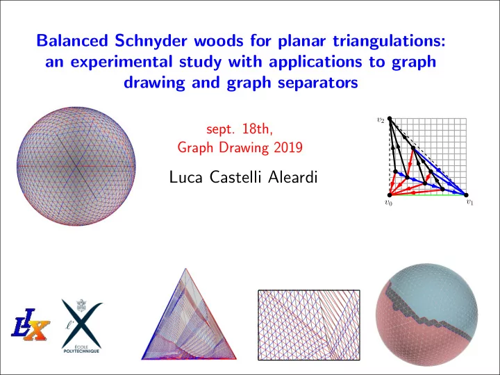
Balanced Schnyder woods for planar triangulations: an experimental - PowerPoint PPT Presentation

Balanced Schnyder woods for planar triangulations: an experimental study with applications to graph drawing and graph separators v 2 sept. 18th, Graph Drawing 2019 Luca Castelli Aleardi v 1 v 0

Planar graphs are ubiquitous (from computational geometry to computer graphics, geometric processing, ...) 3D reconstruction geometric modeling Delaunay triangulation GIS Technology David statue (Stanford’s Digital Michelangelo Project, 2000) Real-world graphs are very regular and far from random or pathological cases regularity measure : we use d 6 , the proportion of degree 6 vertices d 6 ≈ 0 . 11 d 6 ≈ 0 . 28 d 6 ≈ 0 . 50 d 6 ≈ 0 . 82 d 6 ≈ 0 . 99 Delaunay triangulation random planar triang.

Some facts about planar graphs (”As I have known them”) Kuratowski theorem (1930) (cfr Wagner’s theorem, 1937) • G contains neither K 5 nor K 3 , 3 as minors Schnyder woods (’89) • planarity criterion via dimension of partial orders: dim ( G ) ≤ 3 • linear-time grid drawing, with O ( n ) × O ( n ) resolution v 2 Thm (Tutte barycentric method, 1963) Every 3 -connected planar graph G admits a convex representation in R 2 . v 0 v 1 Thm (Koebe-Andreev-Thurston) Thm (Colin de Verdi` ere, 1990) Colin de Verdiere invariant Every planar graph with n vertices is (multiplicity of λ 2 eigenvalue of a generalized laplacian) isomorphic to the intersection graph of n • µ ( G ) ≤ 3 disks in the plane. − 1 4 . . . . . . 0 L G [ i, k ] = { − A G [ i, j ] deg ( v i ) . . . − 1 5 . . . . . . . . . . . . . . . 0 3

Schnyder woods (quick overview) Planar triangulations 3 -connected planar graphs toroidal triangulations [Schnyder ’90] [Felsner ’01] [Goncalves L´ evˆ eque, ’14] genus g triangulations [Castelli Aleardi Fusy Lewiner, ’08] v 2 v 1 v 0

Schnyder woods: (planar) definition [Schnyder ’90] v 2 v 2 v 0 rooted triangulation on v 1 n nodes T 0 , T 1 and T 2 are vertex spanning trees v 1 v 0 D ef A Schnyder wood of a (rooted) planar triangulation is partition of all inner edges into three sets T 0 , T 1 and T 2 , s.t. i) edge are colored and oriented in such a way that each inner nodes has exaclty one outgoing edge of each color ii) colors and orientations around each inner node must respect the local Schnyder condition

Looking for ”nice” Schnyder woods Counting Schnyder woods: (there are an exponential number) ≈ 16 n [Bonichon ’05] # Schnyder woods of triangulations of size n : # planar triangulations of size n : |T n | ≈ 2 3 . 2451 2 . 37 n ≤ max | SW ( T ) | ≤ 3 . 56 n [Felsner Zickfeld ’08] T ∈ T n (count of Schnyder woods of a fixed triangulation) T n := class of planar triangulations of size n SW ( T ) := set of all Schnyder woods of the triangulation T Egalitarian orientations: (only for unconstrained orientations) [Borradaile et al. ’17] ”find an orientation s. t. no vertex is unfairly hit with too many arcs directed into it” Goal : find an edge orientation that minimizes the lexicographic order of indegrees (or minimize maximum indegree)

Balanced Schnyder woods v 2 δ ( v ) = 0 δ ( v ) = (2 − 1) − 1 = 0 δ ( v ) = 1 δ ( v ) = (3 − 0) − 1 = 2 balanced vertex balanced vertex unbalanced vertices v 1 v 0 D ef { max indeg i ( v ) − min indeg i ( v ) if degree ( v ) = 3 k i ∈ { 0 , 1 , 2 } i ∈ { 0 , 1 , 2 } δ ( v ) := vertex defect max indeg i ( v ) − min indeg i ( v ) − 1 otherwwise i ∈ { 0 , 1 , 2 } i ∈ { 0 , 1 , 2 } indeg i ( v ) := # incoming edges of color i A Schnyder wood is balanced if most vertices have a small defect perfectly balanced well balanced strongly unbalanced

Computing balanced Schnyder woods balancedSchnyderWood( T , ( v 0 , v 1 , v 2 ) , k ) Proportion of balanced vertices with our heuristic B = { v 0 , v 1 , v 2 } // initialization T = new int[n] // priority array Q 0 = ∅ , Q 1 = ∅ , . . . Q k − 1 = ∅ // queue initialization Q 0 .addLast ( v 2 ) while( | B | � = { v 0 , v 1 } ) { well balanced let M be the largest index s.t. Q M � = ∅ let v = Q M . poll () minimal Schnyder wood if( v ∈ B and v is free) { let { v l , v j 1 , . . . v j t , v r } be the neighbors of v on B colorOrient ( v ) conquer ( v ) // remove v from B T [ v l ] + + , T [ v r ] + + // increase priority Q max( k − 1 ,T [ v l ]) .addLast ( v l ) strongly unbalanced Q max( k − 1 ,T [ v r ]) .addLast ( v r ) ( d 6 := proportion of Q 0 .addLast ( v j 1 ), . . . , Q 0 .addLast ( v j t ) } degree 6 vertices) } Incremental vertex shelling remove first boundary vertices with priority driven vertex conquest: (Brehm’s diploma thesis) higher number of ingoing edges

Layout quality for Schnyder drawings high values indicates more unbalanced (higher values are better) uniform edge length el edge length metric sphere12k horse Egea δ avg := 1 well balanced (our heuristic) � v δ ( v ) (average vertex defect) n (Fowler and Kobourov, 2012) average percent deviation of edge length � � | l ( e ) − l avg | 1 � el := 1 − e ∈ E | E | max( l avg ,l max − l avg ) l ( e ) := edge length of e

From Schnyder woods to cycle separators choose the best index i and vertex v s.t. { S = P i ( v ) ∪ P i +2 ( v ) ∪ { v } is minimized (Fox-Epstein et al. 2016, Holzer et al. 2009) | A | ≤ 2 A = Int ( R i ( v ) ∪ R i +2 ( v )) 3 n Def ( small balanced cycle separators ) | B | ≤ 2 B = Int ( R i +1 ( v )) 3 n A partition ( A, B, S ) of V ( G ) such that: S defines a simple cycle A and B are balanced: | A | ≤ 2 3 n , | B | ≤ 2 v 6 3 n A the separator is small: | S | ≤ √ 8 m B Boundary size Separator balance n = number of vertices m = number of edges (tests are repated with 200 random choices of the initial seed , the root face) | S | = 0 . 58 √ m | S | = 1 . 32 √ m | S | = 0 . 96 √ m n = 2012 δ 0 = 0 . 543 diam= 202 δ avg = 1 . 153 δ avg = 0 . 931 δ avg = 0 . 921 δ avg = 1 . 18 | S | = 0 . 15 √ m δ 0 = 0 . 485 δ 0 = 0 . 485 δ 0 = 0 . 42 horse Egea cylinder2k n = 8268 δ avg = 1 . 148 n = 20000 | S | = 2 . 34 √ m diam= 59 δ 0 = 0 . 546 diam= 168

From Schnyder woods to cycle separators How the separator quality depends on the balance unbalanced (lower values are better) sphere12k horse Egea Boundary size δ avg := 1 � v δ ( v ) (average vertex defect) n well balanced (our heuristic)

Evaluation of timing costs total timing costs average timings (over 100 executions) ( 100 choice of random seeds) computing balanced Schnyder woods computing Schnyder drawing computing shortest separator seconds Our performances (pure Java , on a core i7-5600 U, 2.60GHz, 1GB Ram): We can process ≈ 1 . 43 M − 1 . 92 M vertices/seconds Metis can process ≈ 0 . 7 M vertices/seconds ( C , on a Intel core i7-5600 2.60GHz) Previous works can process ≈ 0 . 54 M − 0 . 62 M vertices/seconds ( C/C++ , on a Xeon X5650 2.67GHz) (Fox-Epstein et al. 2016, Holzer et al. 2009) Our datasets (several tens of real-world, random and synthetic graphs) Synthetic graphs 3d meshes from aim@shape and Thingi 10k Random triangulations

Thanks

Improving the balance (returning oriented cycles)