
Chapter 7 Dynamic Programming
NEW CS 473: Theory II, Fall 2015 September 15, 2015
7.1 Optimal Triangulations
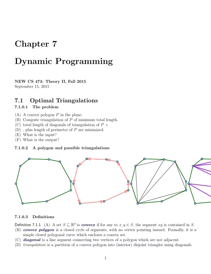
7.1.0.1 The problem (A) A convex polygon P in the plane. (B) Compute triangulation of P of minimum total length. (C) total length of diagonals of triangulation of P + (D) , plus length of perimeter of P are minimized. (E) What is the input? (F) What is the output? 7.1.0.2 A polygon and possible triangulations 7.1.0.3 Definitions Definition 7.1.1. (A) A set S ⊆ Rd is convex if for any to x, y ∈ S, the segment xy is contained in S. (B) convex polygon is a closed cycle of segments, with no vertex pointing inward. Formally, it is a simple closed polygonal curve which encloses a convex set. (C) diagonal is a line segment connecting two vertices of a polygon which are not adjacent. (D) triangulation is a partition of a convex polygon into (interior) disjoint triangles using diagonals. 1