Dynamic Programming Dynamic Programming Steps. 9 View the problem - - PDF document

Dynamic Programming

• Steps.

9View the problem solution as the result of a sequence

• f decisions.

9Obtain a formulation for the problem state. 9Verify that the principle of optimality holds. 9Set up the dynamic programming recurrence equations. 9Solve these equations for the value of the optimal solution. Perform a traceback to determine the optimal solution.

Dynamic Programming

• When solving the dynamic programming

recurrence recursively, be sure to avoid the recomputation of the optimal value for the same problem state.

• To minimize run time overheads, and hence

to reduce actual run time, dynamic programming recurrences are almost always solved iteratively (no recursion).

0/1 Knapsack Recurrence

• If wn <= y, f(n,y) = pn.
• If wn > y, f(n,y) = 0.
• When i < n

f(i,y) = f(i+1,y) whenever y < wi. f(i,y) = max{f(i+1,y), f(i+1,y-wi) + pi}, y >= wi.

• Assume the weights and capacity are integers.
• Only f(i,y)s with 1 <= i <= n and 0 <= y <= c

are of interest.

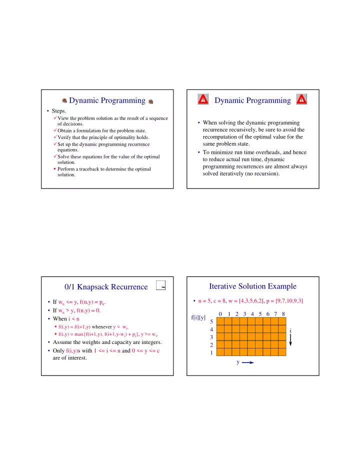
Iterative Solution Example

• n = 5, c = 8, w = [4,3,5,6,2], p = [9,7,10,9,3]

y 5 4 3 2 1 f[i][y] 1 2 3 4 5 6 7 8 i

Compute f[5][*]

• n = 5, c = 8, w = [4,3,5,6,2], p = [9,7,10,9,3]

y 5 4 3 2 1 f[i][y] 1 2 3 4 5 6 7 8 i

3 3 3 3 3 3 3

Compute f[4][*]

• n = 5, c = 8, w = [4,3,5,6,2], p = [9,8,10,9,3]

y 5 4 3 2 1 f[i][y] 1 2 3 4 5 6 7 8 i

3 3 3 3 3 3 3 3 3 3 3 9 9 12

f(i,y) = max{f(i+1,y), f(i+1,y-wi) + pi}, y >= wi

Compute f[3][*]

• n = 5, c = 8, w = [4,3,5,6,2], p = [9,8,10,9,3]

y 5 4 3 2 1 f[i][y] 1 2 3 4 5 6 7 8 i

3 3 3 3 3 3 3 3 3 3 3 9 9 12 3 3 3 10 10 13 13

f(i,y) = max{f(i+1,y), f(i+1,y-wi) + pi}, y >= wi

Compute f[2][*]

• n = 5, c = 8, w = [4,3,5,6,2], p = [9,8,10,9,3]

y 5 4 3 2 1 f[i][y] 1 2 3 4 5 6 7 8 i

3 3 3 3 3 3 3 3 3 3 3 9 9 12 3 3 3 10 10 13 13 3 8 8 11 11 13 18

f(i,y) = max{f(i+1,y), f(i+1,y-wi) + pi}, y >= wi

Compute f[1][c]

• n = 5, c = 8, w = [4,3,5,6,2], p = [9,8,10,9,3]

y 5 4 3 2 1 f[i][y] 1 2 3 4 5 6 7 8 i

3 3 3 3 3 3 3 3 3 3 3 9 9 12 3 3 3 10 10 13 13 3 8 8 11 11 13 18 18

f(i,y) = max{f(i+1,y), f(i+1,y-wi) + pi}, y >= wi

Iterative Implementation

// initialize f[n][] int yMax = Math.min(w[n] - 1, c); for (int y = 0; y <= yMax; y++) f[n][y] = 0; for (int y = w[n]; y <= c; y++) f[n][y] = p[n];

Iterative Implementation

// compute f[i][y], 1 < i < n for (int i = n - 1; i > 1; i--) { yMax = Math.min(w[i] - 1, c); for (int y = 0; y <= yMax; y++) f[i][y] = f[i + 1][y]; for (int y = w[i]; y <= c; y++) f[i][y] = Math.max(f[i + 1][y], f[i + 1][y - w[i]] + p[i]); }

Iterative Implementation

// compute f[1][c] f[1][c] = f[2][c]; if (c >= w[1]) f[1][c] = Math.max(f[1][c], f[2][c-w[1]] + p[1]); }

Time Complexity

• O(cn).
• Same as for the recursive version with no

recomputations.

• Iterative version is expected to run faster

because of lower overheads.

No checks to see if f[i][j] already computed (but all f[i][j] are computed). Method calls replaced by for loops.

Traceback

• n = 5, c = 8, w = [4,3,5,6,2], p = [9,8,10,9,3]

y 5 4 3 2 1 f[i][y] 1 2 3 4 5 6 7 8 i

3 3 3 3 3 3 3 3 3 3 3 9 9 12 3 3 3 10 10 13 13 3 8 8 11 11 13 18 18

f[1][8] = f[2][8] => x1 = 0

Traceback

• n = 5, c = 8, w = [4,3,5,6,2], p = [9,8,10,9,3]

y 5 4 3 2 1 f[i][y] 1 2 3 4 5 6 7 8 i

3 3 3 3 3 3 3 3 3 3 3 9 9 12 3 3 3 10 10 13 13 3 8 8 11 11 13 18 18

f[2][8] != f[3][8] => x2 = 1

10

Traceback

• n = 5, c = 8, w = [4,3,5,6,2], p = [9,8,10,9,3]

y 5 4 3 2 1 f[i][y] 1 2 3 4 5 6 7 8 i

3 3 3 3 3 3 3 3 3 3 3 9 9 12 3 3 3 10 10 13 13 3 8 8 11 11 13 18 18

f[3][5] != f[4][5] => x3 = 1

Traceback

• n = 5, c = 8, w = [4,3,5,6,2], p = [9,8,10,9,3]

y 5 4 3 2 1 f[i][y] 1 2 3 4 5 6 7 8 i

3 3 3 3 3 3 3 3 3 3 3 9 9 12 3 3 3 10 10 13 13 3 8 8 11 11 13 18 18

f[4][0] = f[5][0] => x4 = 0

Traceback

• n = 5, c = 8, w = [4,3,5,6,2], p = [9,8,10,9,3]

y 5 4 3 2 1 f[i][y] 1 2 3 4 5 6 7 8 i

3 3 3 3 3 3 3 3 3 3 3 9 9 12 3 3 3 10 10 13 13 3 8 8 11 11 13 18 18

f[5][0] = 0 => x5 = 0

Complexity Of Traceback

• O(n)

Matrix Multiplication Chains

• Multiply an m x n matrix A and an n x p matrix

B to get an m x p matrix C. k = 1 n C(i,j) = A(i,k) * B(k,j)

• We shall use the number of multiplications as
• ur complexity measure.
• n multiplications are needed to compute one

C(i,j).

• mnp multiplicatons are needed to compute all

mp terms of C.

Matrix Multiplication Chains

• Suppose that we are to compute the product X*Y*Z of

three matrices X, Y and Z.

• The matrix dimensions are:

X:(100 x 1), Y:(1 x 100), Z:(100 x 1)

• Multiply X and Y to get a 100 x 100 matrix T.

100 * 1 * 100 = 10,000 multiplications.

• Multiply T and Z to get the 100 x 1 answer.

100 * 100 * 1 = 10,000 multiplications.

• Total cost is 20,000 multiplications.
• 10,000 units of space are needed for T.

Matrix Multiplication Chains

• The matrix dimensions are:

X:(100 x 1) Y:(1 x 100) Z:(100 x 1)

• Multiply Y and Z to get a 1 x 1 matrix T.

1 * 100 * 1 = 100 multiplications.

• Multiply X and T to get the 100 x 1 answer.

100 * 1 * 1 = 100 multiplications.

• Total cost is 200 multiplications.
• 1 unit of space is needed for T.

Product Of 5 Matrices

• Some of the ways in which the product of 5 matrices

may be computed.

A*(B*(C*(D*E))) right to left (((A*B)*C)*D)*E left to right (A*B)*((C*D)*E) (A*B)*(C*(D*E)) (A*(B*C))*(D*E) ((A*B)*C)*(D*E)

Find Best Multiplication Order

• Number of ways to compute the product of q

matrices is O(4q/q1.5).

• Evaluating all ways to compute the product

takes O(4q/q0.5) time.

An Application

• Registration of pre- and post-operative 3D brain

MRI images to determine volume of removed tumor.

3D Registration 3D Registration

• Each image has 256 x 256 x 256 voxels.
• In each iteration of the registration algorithm, the

product of three matrices is computed at each voxel … (12 x 3) * (3 x 3) * (3 x 1)

• Left to right computation => 12 * 3 * 3 + 12 * 3*1

= 144 multiplications per voxel per iteration.

• 100 iterations to converge.

3D Registration

• Total number of multiplications is about 2.4 *

1011.

• Right to left computation => 3 * 3*1 + 12 * 3 * 1

= 45 multiplications per voxel per iteration.

• Total number of multiplications is about 7.5 *

1010.

• With 108 multiplications per second, time is 40

min vs 12.5 min.