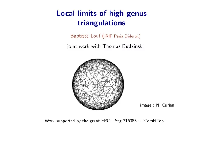
SLIDE 1 Local limits of high genus triangulations
Baptiste Louf (IRIF Paris Diderot)
Work supported by the grant ERC – Stg 716083 – “CombiTop”
joint work with Thomas Budzinski
image : N. Curien
SLIDE 2 Maps and triangulations
= =
Map = embedding up to homeomorphism of a connected multigraph (loops and multiple edges allowed) in a compact connected
Rooted = an oriented edge is distinguished
SLIDE 3 Maps and triangulations
= =
Map = embedding up to homeomorphism of a connected multigraph (loops and multiple edges allowed) in a compact connected
Rooted = an oriented edge is distinguished Genus g of the map = genus of the surface = # of handles
SLIDE 4 Maps and triangulations
= =
Map = embedding up to homeomorphism of a connected multigraph (loops and multiple edges allowed) in a compact connected
Rooted = an oriented edge is distinguished Genus g of the map = genus of the surface = # of handles Triangulation = all faces of degree 3
SLIDE 5
What does a triangulation look like around the root ?
How similar are two triangulations locally ?
SLIDE 6
What does a triangulation look like around the root ?
How similar are two triangulations locally ? The local distance : dloc(T, T ′) = (1 + sup{r|Br(T) = Br(T ′)})−1
SLIDE 7 The limit (in law) w.r.t dloc is called the local limit. Question : let (Tn) be a sequence of random triangulations, whose size → ∞, is there a local limit ? What does it look like ? [Angel, Schramm ’02] : uniform planar triangulations converge to an infinite triangulation called the Uniform Infinite Planar Triangulation (UIPT).
What does a (large, random) triangulation look like around the root ?
image : I. Kortchemski
SLIDE 8 Properties of the UIPT
Spatial Markov property : P(t ⊂ T) = Cpλ|v|
c
⊂
p = 7, |v| = 9
SLIDE 9 Properties of the UIPT
Spatial Markov property : P(t ⊂ T) = Cpλ|v|
c
⊂
λc = rcv of the series of planar triangulations ! p = 7, |v| = 9
SLIDE 10 Properties of the UIPT
Spatial Markov property : P(t ⊂ T) = Cpλ|v|
c
⊂
λc = rcv of the series of planar triangulations ! Peeling process : Discover T step by step, unveil triangles. p = 7, |v| = 9
SLIDE 11 Properties of the UIPT
Spatial Markov property : P(t ⊂ T) = Cpλ|v|
c
⊂
λc = rcv of the series of planar triangulations ! Peeling process : Discover T step by step, unveil triangles. = p = 7, |v| = 9
SLIDE 12 Properties of the UIPT
Spatial Markov property : P(t ⊂ T) = Cpλ|v|
c
⊂
λc = rcv of the series of planar triangulations ! Peeling process : Discover T step by step, unveil triangles. λc = (x2)
p = 7, |v| = 9
SLIDE 13 The PSHIT
Introduced by Curien in 2012 Defined in the same way as the UIPT, by with λ ∈]0, λc]. For λ < λc, has an hyperbolic flavour : the ”average degree” of a vertex is higher than 6 (the value in a regular planar triangulation), the balls have exponential growth, . . .
image : N. Curien
SLIDE 14
Question : Can the PSHITs be interpreted as local limits ?
SLIDE 15 A conjecture
image : N. Curien
Let gn
n → θ with θ ∈ [0, 1 2[.
Let (Tn) be a sequence of random triangulations, such that Tn is drawn uniformly among all triangulations of genus gn with 2n triangles. Conjecture [Benjamini, Curien ’12] : (Tn) has a local limit, and it is a PSHIT of parameter λ, with λ a function of θ. For gn constant, the limit is the UIPT (well known,but never written anywhere).
SLIDE 16 A conjecture
A similar result [Angel, Chapuy, Curien, Ray ’13] : the local limit of one-faced maps of high genus is an infinite hyperbolic tree
image : ACCR image : N. Curien
Let gn
n → θ with θ ∈ [0, 1 2[.
Let (Tn) be a sequence of random triangulations, such that Tn is drawn uniformly among all triangulations of genus gn with 2n triangles. Conjecture [Benjamini, Curien ’12] : (Tn) has a local limit, and it is a PSHIT of parameter λ, with λ a function of θ. For gn constant, the limit is the UIPT (well known,but never written anywhere).
SLIDE 17
For fixed genus . . .
The intuition behind the conjecture
SLIDE 18
For fixed genus . . .
The intuition behind the conjecture
SLIDE 19
For fixed genus . . .
The intuition behind the conjecture
SLIDE 20
For fixed genus . . .
The intuition behind the conjecture
SLIDE 21
For fixed genus . . .
The intuition behind the conjecture
SLIDE 22
For fixed genus . . . In the limit we see the ”tangent plane of an infinite triangulation”.
The intuition behind the conjecture
SLIDE 23
For fixed genus . . . In the limit we see the ”tangent plane of an infinite triangulation”. When the genus increases linearly with the size, in the end we don’t see the genus but we still ”feel the curvature”
The intuition behind the conjecture
SLIDE 24 Our result
Theorem [Budzinski, L. ’18+] : the conjecture
- f Benjamini and Curien is true.
SLIDE 25 First idea : Obtain precise asymptotics for τ(n, g) (the number of triangulations of genus g with 2n triangles) as g
n → θ
SLIDE 26 First idea : Obtain precise asymptotics for τ(n, g) (the number of triangulations of genus g with 2n triangles) as g
n → θ
TOO HARD
SLIDE 27
Outline of the proof :
1) Tightness (+ planarity and one-endedness) 2) Every possible limit is a PSHIT with random parameter Λ 3) Λ is deterministic and depends only on θ → every subsequence has a converging subsubsequence
SLIDE 28
Bonus : asymptotics ! τ(n, gn) τ(n − 1, gn) → c(θ) τ(n, gn) = n2gn exp(nf(θ) + o(n))
SLIDE 29 What’s next ?
More geometric info on high genus maps ? What happens when g
n → 1 2 ?
Maps decorated with ”matter” ? Boltzmann maps Diameter of high genus maps (= log n, [Chapuy, L., Marzouk ’19+])
SLIDE 30
Thank you !