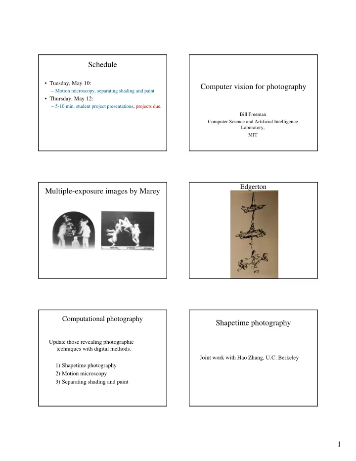
Schedule Tuesday, May 10: Computer vision for photography Motion - - PDF document

1

Schedule

• Tuesday, May 10:

– Motion microscopy, separating shading and paint

• Thursday, May 12:

– 5-10 min. student project presentations, projects due.

Computer vision for photography

Bill Freeman Computer Science and Artificial Intelligence Laboratory, MIT

Multiple-exposure images by Marey

Edgerton Computational photography

Update those revealing photographic techniques with digital methods. 1) Shapetime photography 2) Motion microscopy 3) Separating shading and paint

Shapetime photography

Joint work with Hao Zhang, U.C. Berkeley

2

Video frames Multiple- exposure Layer- By-Time Shape- Time

“how to sew”

3

Shape-Time composite “inside-out” Input sequence

Insert pictures describing zcam, and initial results

Motion Magnification

Ce Liu Antonio Torralba William T. Freeman Fredo Durand Edward H. Adelson

Goal

A microscope for motion

You focus the microscope by specifying which motions to magnify, and by how much; the motion microscope then re-renders the input sequence with the desired motions magnified.

The naïve solution has artifacts

Original sequence Naïve motion magnification Amplified dense Lukas-Kanade optical flow. Note artifacts at occlusion boundaries.

Motion magnification flowchart

Input raw video sequence Register frames Find feature point trajectories Cluster trajectories Interpolate dense

• ptical flow

Segment flow into layers Magnify selected layer, Fill-in textures Render magnified video sequence

Layer-based motion analysis

1 2 3 4 5 6 7

4

1 Video Registration

• To find a reliable set of feature points that are

“still” in the sequence

– Detect and track feature points – Estimate the affine motion from the reference frame to each of the rest frames – Select feature points that are inliers through all the frames – Affine warping based on the inliers

Inliers (red) and outliers (blue) Registration results 2 Find feature point trajectories

• An EM algorithm to find both trajectory and region of

support for each feature point

– E-step: to use the variance of matching score to compute the weight of the neighboring pixels – M-step: to track feature point based on the region of support

• The following feature points are pruned

– Occluded (matching error) – Textureless (motion coherence) – Static (zero motion)

Learned regions of support for features Robust feature point tracking

5

Minimal SSD match to find feature point trajectories

Use EM to find regions of support and prune low-likelihood trajectories

3 Trajectory clustering

We need to cluster trajectories belonging to the same

• bject, despite:

Points have different appearances Undergo very small motions, of varying amplitudes and directions

Vx Vy time time Vy Vx

3 Compatibility function used to group feature point trajectories

ρn,m: compatibility between the nth and mth point trajectories. vx(n,k): the displacement, relative to the reference frame, of the nth feature point in the kth frame. Using the ρn,m compatibilities, cluster the point trajectories using normalized cuts.

Clustering results 4 Dense optical flow field interpolation

• For each layer (cluster) a dense optical flow field

(per pixel) is interpolated

• Use local weighted linear regression to interpolate

between feature point trajectories.

Clustered feature point trajectories Dense trajectories interpolated for each cluster

6

5 Segment flow into layers

• Assign each pixel to a motion cluster layer, using four

cues:

– Motion likelihood – Color likelihood – Spatial connectivity – Temporal coherence

• Energy minimization using graph cuts

Motion segmentation results

Note we have 2 special layers: the background layer (gray), and the outlier layer (black).

6, 7 Magnification, texture fill-in and rendering

• Amplify the motion of the selected layers by warping the reference

image pixels accordingly.

• Render unselected layers without magnification.
• Fill-in holes revealed in background layer using Efros-Leung texture

synthesis

• Directly pass-through pixel values of the outlier layer.

Summary of motion magnification steps

Results

• Demo

Layered representation

7

Is the signal really in the video? (yes)

Original Magnified 25 frames

Swingset details

Beam bending Proper handing

• f occlusions

Artifact

Bookshelf

44 frames 480x640 pixels time time Original Magnified

Bookshelf deforms less, further from force

44 frames 480x640 pixels time time Original Magnified

Outtakes from imperfect segmentations

8

Breathing Mike

Original sequence…

Breathing Mike

Feature points 2 clusters 4 clusters 8 clusters

Breathing Mike

Sequence after magnification…

Standing Mike

Sequence after magnification…

Crane Crane

Feature points 2 clusters 4 clusters 8 clusters

9

Crane

Things can go horribly wrong sometimes…

What next

• Continue improving the motion segmentation.

– Motion magnification is “segmentation artifact amplification”—a good test bed.

• Real applications

– Videos of inner ear – Connections with mechanical engineering dept.

• Generalization: amplifying small differences in

motion.

– What’s up with Tiger Woods’ golf swing, anyway?