Scatter Plots MPM1D: Principles of Mathematics Recap A student - - PDF document

a n a l y z i n g d a t a

MPM1D: Principles of Mathematics

Trends in Data: Interpolation and Extrapolation

• J. Garvin

Slide 1/17

a n a l y z i n g d a t a

Scatter Plots

Recap

A student records the times it takes for a chemical reaction to occur when a certain mass of chemical is added to a solution in the table below. Identify the independent and dependent variables, and create a scatter plot of the data. Mass (g) 10 15 18 25 32 44 48 55 Time (sec) 8.4 8.2 8.1 7.5 7.3 7.0 6.8 6.8 Since the time for a reaction to occur depends on the mass

• f the chemical added to the solution, time is the dependent

variable and mass is the independent variable. As such,the vertical axis will measure time and the horizontal axis will measure mass.

• J. Garvin — Trends in Data: Interpolation and Extrapolation

Slide 2/17

a n a l y z i n g d a t a

Scatter Plots

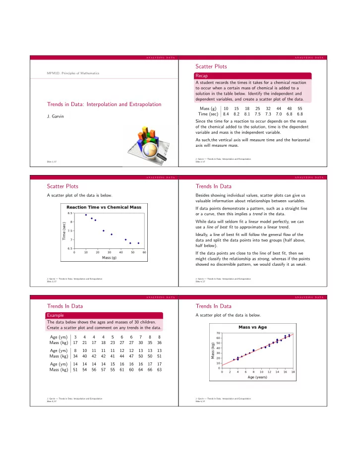
A scatter plot of the data is below.

• J. Garvin — Trends in Data: Interpolation and Extrapolation

Slide 3/17

a n a l y z i n g d a t a

Trends In Data

Besides showing individual values, scatter plots can give us valuable information about relationships between variables. If data points demonstrate a pattern, such as a straight line

• r a curve, then this implies a trend in the data.

While data will seldom fit a linear model perfectly, we can use a line of best fit to approximate a linear trend. Ideally, a line of best fit will follow the general flow of the data and split the data points into two groups (half above, half below). If the data points are close to the line of best fit, then we might classify the relationship as strong, whereas if the points showed no discernible pattern, we would classify it as weak.

• J. Garvin — Trends in Data: Interpolation and Extrapolation

Slide 4/17

a n a l y z i n g d a t a

Trends In Data

Example

The data below shows the ages and masses of 30 children. Create a scatter plot and comment on any trends in the data. Age (yrs) 3 4 4 4 5 6 6 7 8 8 Mass (kg) 17 21 17 18 23 27 27 30 35 36 Age (yrs) 8 10 11 11 11 12 12 13 13 13 Mass (kg) 34 40 42 42 41 44 47 50 50 51 Age (yrs) 14 14 14 14 15 16 16 16 17 17 Mass (kg) 51 54 56 57 55 61 60 64 66 63

• J. Garvin — Trends in Data: Interpolation and Extrapolation

Slide 5/17

a n a l y z i n g d a t a

Trends In Data

A scatter plot of the data is below.

• J. Garvin — Trends in Data: Interpolation and Extrapolation

Slide 6/17

a n a l y z i n g d a t a

Trends In Data

There appears to be a linear trend in the data, as shown by the line in red. As a child’s age increases, his/her mass also increases. Since all data points are fairly close to the line of best fit, this suggests a strong relationship between a child’s age and his/her mass. There could be other factors that influence a child’s mass (e.g. diet, fitness, genetics, health) as well, and these would need to be considered before drawing any firm conclusions.

• J. Garvin — Trends in Data: Interpolation and Extrapolation

Slide 7/17

a n a l y z i n g d a t a

Trends In Data

Example

A teacher uses software to compare the amount of time spent doing homework per week, and a score on a recent mathematics test. Comment on any trends in the data.

• J. Garvin — Trends in Data: Interpolation and Extrapolation

Slide 8/17

a n a l y z i n g d a t a

Trends In Data

There is a general trend in the data that as the number of hours of homework done each week increases, a student’s test score increases. This relationship is not very strong, since a number of data points are fairly far from the line. This could be due to several reasons including general mathematical ability, familiarity with concepts, extra-curricular involvement, and so on. As such, there appears to be some link between an increased time spent doing homework time and a high score on a test, but there are probably other factors that influence the data.

• J. Garvin — Trends in Data: Interpolation and Extrapolation

Slide 9/17

a n a l y z i n g d a t a

Trends In Data

Example

Suppose that the teacher in the previous example identifies the following two students as outliers:

• 0 hours on homework, 94% on test: student has recently

moved from a province where the same material was taught last year,

• 14 hours on homework, 57% on test: student has severe

dyscalculia, spends four nights per week working with math tutor. Discuss any arguments in favour of, or against, removing these two students from the sample. What effect(s) would removing them have on the trend?

• J. Garvin — Trends in Data: Interpolation and Extrapolation

Slide 10/17

a n a l y z i n g d a t a

Trends In Data

The teacher may wish to remove the students from the sample because they may not be representative of the class as a whole – one has a great deal of experience with what is “new” material to others, while the other has difficulty processing mathematical concepts and logic. On the other hand, it is possible that there are other students in the class that have similar backgrounds and the teacher simply does not know about them. In this case, the teacher may wish to include them. If the two students were removed from the sample, the line

• f best fit would better approximate the data, since the
• utliers would no longer have any influence.
• J. Garvin — Trends in Data: Interpolation and Extrapolation

Slide 11/17

a n a l y z i n g d a t a

Trends In Data

A graph of the data with the outliers removed is below, showing a better fit to the linear model.

• J. Garvin — Trends in Data: Interpolation and Extrapolation

Slide 12/17

a n a l y z i n g d a t a

Trends In Data

Bar graphs and line graphs are also used to display information, but they are used for displaying trends shown by a single variable instead. Often, bar and line graphs display how a variable changes

• ver time, but this is not the only case.

Both bar graphs and line graphs display the same information, but in different forms, and are sometimes used interchangeably.

• J. Garvin — Trends in Data: Interpolation and Extrapolation

Slide 13/17

a n a l y z i n g d a t a

Trends In Data

Example

The bar graph below shows the number of new members to an online gaming service over time. Subscriber data from 2015 has been lost. Comment on any trends.

• J. Garvin — Trends in Data: Interpolation and Extrapolation

Slide 14/17

a n a l y z i n g d a t a

Trends In Data

While the number of new members increases each year, it does not appear to be linear – a trend line would curve upward as the year increases. How many new members could there have been in 2015? How can we obtain an estimate? Interpolation is when a trend is used to determine a value that falls within a data set, whereas extrapolation is when values are found outside of a data set. If we can identify a pattern in the data, then we can use its properties to predict values both within and outside of the data set.

• J. Garvin — Trends in Data: Interpolation and Extrapolation

Slide 15/17

a n a l y z i n g d a t a

Trends In Data

Example

Using the new member information from the previous example, predict the number of new member subscriptions in 2015 and in 2017. Since the number of new members seems to double each year, we can interpolate a value for 2015 by either multiplying the number from 2014 by two, or by dividing the number from 2016 by two. This gives a range of between 25 000 and 28 000 new members. We can extrapolate a value for 2016 by doubling the number, giving us an estimate of approximately 100 000 new members.

• J. Garvin — Trends in Data: Interpolation and Extrapolation

Slide 16/17

a n a l y z i n g d a t a

Questions?

• J. Garvin — Trends in Data: Interpolation and Extrapolation

Slide 17/17