s n
play

S N element and should be in the Gaussian surface region - PowerPoint PPT Presentation

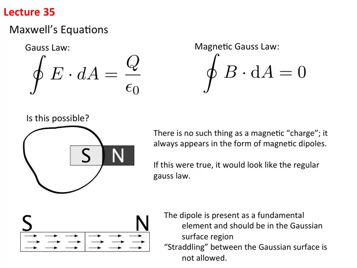
Lecture 35 Maxwells Equa-ons Magne-c Gauss Law: Gauss Law: I E dA = Q I B d A = 0 0 Is this possible? There is no such thing as a magne-c


  1. Lecture ¡35 ¡ Maxwell’s ¡Equa-ons ¡ Magne-c ¡Gauss ¡Law: ¡ Gauss ¡Law: ¡ I E · dA = Q I B · d A = 0 ✏ 0 Is ¡this ¡possible? ¡ There ¡is ¡no ¡such ¡thing ¡as ¡a ¡magne-c ¡“charge”; ¡it ¡ always ¡appears ¡in ¡the ¡form ¡of ¡magne-c ¡dipoles. ¡ S N ¡ If ¡this ¡were ¡true, ¡it ¡would ¡look ¡like ¡the ¡regular ¡ gauss ¡law. ¡ The ¡dipole ¡is ¡present ¡as ¡a ¡fundamental ¡ S N ¡element ¡and ¡should ¡be ¡in ¡the ¡Gaussian ¡ ¡surface ¡region ¡ “Straddling” ¡between ¡the ¡Gaussian ¡surface ¡is ¡ ¡not ¡allowed. ¡

  2. Maxwell’s ¡Equa-ons ¡– ¡con-nued... ¡ Ampere’s ¡Law ¡ I Z B · d l = µ 0 I Current ¡running ¡through ¡ the ¡surface ¡where ¡the ¡rim ¡ of ¡the ¡surface ¡= ¡path ¡ E (think ¡of ¡the ¡surface ¡as ¡a ¡soap ¡bubble ¡filament) ¡ Mathema-cally, ¡the ¡film ¡ doesn’t ¡need ¡to ¡be ¡flat ¡ E = Q/A , ¡ Q = ✏ 0 EA ✏ 0 Charge ¡build-­‑up ¡on ¡the ¡plate ¡generates ¡an ¡electric ¡flux ¡ Responsible ¡for ¡piercing ¡the ¡surface ¡defined ¡by ¡the ¡rim ¡ dQ d Φ E (Virtual ¡current, ¡or ¡the ¡displacement ¡current ¡I D , ¡to ¡be ¡ dt = ✏ 0 added ¡to ¡“I” ¡in ¡Amp-­‑Maxwell ¡Law) ¡ dt (For ¡par-al ¡piercing, ¡refer ¡to ¡Fig(mi) ¡24.5) ¡

  3. Discussion ¡of ¡Ch24.Hw1.001 ¡ Set-­‑up: ¡ , ¡increasing ¡ E ext = uniform Apply ¡Ampere-­‑Maxwell ¡Law: ¡ R 2 π RB p = µ 0 [ NI toroid + I DC ] P ¡ (2) ¡ I (1) ¡ I d Φ E ✏ 0 Cau-on, ¡check ¡contribu-ons ¡of: ¡ ¡ dt ⇢ CW ⇢ CW (1) (2) CCW CCW Exercise: ¡Check ¡various ¡cases: ¡ ⇢ CW Clicker ¡1: ¡ Contrib. ¡of ¡(1) ¡ Contrib. ¡of ¡(2) ¡ ~ E ⊗ CCW correct ¡ 1) ¡ CW ¡ CW ¡ ⇢ CW 2) ¡ CCW ¡ CW ¡ ~ 3) ¡ CW ¡ CCW ¡ E � CCW 4) ¡ CCW ¡ CCW ¡ 3 ¡

  4. One ¡Dimensional ¡EM ¡Pulse ¡ We ¡use ¡the ¡following ¡example ¡used ¡by ¡Professor ¡Feynman ¡to ¡ illustrate ¡some ¡of ¡the ¡proper-es ¡of ¡EM ¡pulse. ¡The ¡geometry ¡of ¡the ¡ setup ¡is ¡shown ¡in ¡fig ¡35.2 ¡and ¡fig ¡35.3 ¡ A ¡warm ¡up. ¡There ¡is ¡the ¡presence ¡of ¡a ¡current ¡sheet ¡at ¡x ¡= ¡0 ¡in ¡the ¡ yz-­‑plane. ¡If ¡the ¡current ¡I ¡is ¡constant, ¡it ¡generates ¡a ¡familiar ¡B ¡pabern ¡ y shown ¡in ¡fig ¡35.4 ¡ � ⊗ � I ⊗ X � ⊗ z � ⊗ For ¡x ¡> ¡0, ¡B-­‑lines ¡are ¡poin-ng ¡in ¡the ¡–z ¡direc-on. ¡For ¡x ¡< ¡0, ¡B ¡lines ¡are ¡ in ¡the ¡+z ¡direc-on. ¡ Now ¡we ¡proceed ¡to ¡discuss ¡the ¡genera-on ¡of ¡1D-­‑EM ¡pulse ¡in ¡steps. ¡

  5. Step ¡1: ¡Instead ¡of ¡having ¡a ¡steady ¡current, ¡we ¡turn ¡on ¡the ¡current ¡at ¡t ¡= ¡0. ¡ ¡Here ¡ there ¡is ¡no ¡B-­‑pabern ¡before ¡t ¡= ¡0. ¡The ¡pabern ¡immediately ¡setups ¡when ¡t ¡> ¡0. ¡First, ¡ the ¡B ¡pabern ¡is ¡created ¡in ¡the ¡proximity ¡of ¡x ¡= ¡0. ¡As ¡t ¡increases ¡there ¡is ¡the ¡spread ¡ both ¡in ¡x ¡> ¡0 ¡and ¡in ¡x ¡< ¡0 ¡direc-on ¡with ¡a ¡speed ¡of ¡v. ¡The ¡goal ¡of ¡this ¡exercise ¡is ¡to ¡ use ¡fig ¡35.2 ¡and ¡fig ¡35.3 ¡determine ¡v. ¡ ¡ Step ¡2: ¡In ¡fig ¡35.21 ¡and ¡fig ¡35.2b ¡define ¡the ¡closed ¡path ¡12341. ¡The ¡loop ¡is ¡in ¡the ¡xy ¡ plane ¡at ¡some ¡z ¡value. ¡We ¡view ¡how ¡the ¡flux ¡grows ¡within ¡the ¡window. ¡As ¡shown ¡ in ¡Fig ¡35.2b, ¡the ¡B-­‑flux ¡in ¡the ¡window ¡increases, ¡as ¡the ¡flux ¡expands ¡to ¡the ¡right. ¡ The ¡flux ¡is ¡defined ¡by ¡ φ B = Bhx = Bhvt

  6. Lenz ¡rule ¡states ¡as ¡the ¡B ¡flux ¡into ¡the ¡window ¡increases, ¡there ¡must ¡ be ¡B ind , ¡the ¡induced ¡B, ¡poin-ng ¡out ¡of ¡the ¡loop, ¡which ¡opposes ¡the ¡ increase ¡of ¡the ¡ingoing ¡flux. ¡B ind ¡is ¡caused ¡by ¡CCW ¡emf ¡induced. ¡ ¡ The ¡Faraday’s ¡Law ¡using ¡the ¡closed ¡path ¡12341 ¡gives: ¡ ¡ E ind = E ind h = d φ B (1) ¡ = Bhv, or E ind = Bv ¡ dt Step ¡3: ¡E ind ¡in ¡step ¡2 ¡is ¡the ¡E ¡field ¡of ¡the ¡EM ¡pulse ¡discussed ¡in ¡Sec. ¡ 24.2 ¡in ¡the ¡text. ¡One ¡sees ¡that ¡E ¡x ¡B ¡for ¡the ¡present ¡case ¡is ¡along ¡to ¡ the ¡right. ¡We ¡proceed ¡to ¡shown ¡that ¡Ampere-­‑Maxwell ¡law ¡(AM-­‑law) ¡ leads ¡to ¡an ¡addi-onal ¡rela-onship ¡between ¡E ¡and ¡B ¡which ¡will ¡enable ¡ us ¡to ¡determine ¡v. ¡

  7. Consider ¡the ¡AM-­‑loop ¡12561 ¡shown ¡in ¡(a) ¡and ¡(b) ¡of ¡Fig35.3. ¡Fig35.3a ¡ shows ¡the ¡front ¡view ¡where ¡the ¡loop ¡is ¡at ¡the ¡top. ¡Fig35.3b ¡shows ¡the ¡ top ¡view ¡of ¡the ¡loop. ¡AM-­‑law ¡states: ¡ ¡ � � � � dEbx I d � E ¡ ¡ ¡ ¡ ¡ ¡ ¡ ¡ ¡ ¡ ¡ ¡or ¡ � � � � Bb = ✏ 0 µ 0 , or B = ✏ 0 µ 0 Ev B · dl � = ✏ 0 µ 0 � � � � dt dt ¡ � � � path ¡ This ¡combined ¡with ¡(1) ¡E ¡= ¡Bv ¡leads ¡to ¡ ¡ 1 ≈ 3 × 10 8 m/s B = ✏ 0 µ 0 ( Bv ) v, or v = ¡ √ ✏ 0 µ 0 ¡ Thus ¡EM ¡pulse ¡travels ¡in ¡free ¡space ¡with ¡an ¡universal ¡speed, ¡the ¡speed ¡ of ¡light. ¡

  8. Recap: ¡ Propaga-on ¡of ¡EM ¡waves: ¡ gives ¡the ¡direc-on ¡of ¡propaga-on ¡ 1. ¡ ¡ E ⊥ B , ¡ E × B E = vB 1 2. ¡ ¡ Universal ¡Speed ¡ v = (in ¡a ¡vacuum) ¡ √ µ 0 ✏ 0 All ¡light ¡is ¡an ¡EM ¡wave, ¡and ¡travels ¡with ¡the ¡same ¡speed ¡ 3. ¡ ¡ E = cB Reflec-on: ¡c ¡is ¡the ¡speed ¡of ¡the ¡“wavefront” ¡ Field ¡has ¡a ¡boundary. ¡ ¡This ¡boundary ¡travels ¡ with ¡v ¡= ¡c ¡in ¡vacuum. ¡ The ¡wave ¡shape ¡is ¡ini-ated ¡by ¡the ¡t-­‑dependence ¡of ¡the ¡source. ¡ For ¡sinusoidal ¡current: ¡ E B The ¡squares ¡are ¡ rounded ¡off ¡ B E

Download Presentation
Download Policy: The content available on the website is offered to you 'AS IS' for your personal information and use only. It cannot be commercialized, licensed, or distributed on other websites without prior consent from the author. To download a presentation, simply click this link. If you encounter any difficulties during the download process, it's possible that the publisher has removed the file from their server.

Recommend


More recommend