[PPT] - Routing to every destination in the network Suppose you want to PowerPoint Presentation

SLIDE 1

1

Routing

An Engineering Approach to Computer Networking

What is it?

Process of finding a path from a source

to every destination in the network

Suppose you want to connect to

Antarctica from your desktop

– what route should you take? – does a shorter route exist? – what if a link along the route goes down? – what if you’re on a mobile wireless link?

Routing deals with these types of issues

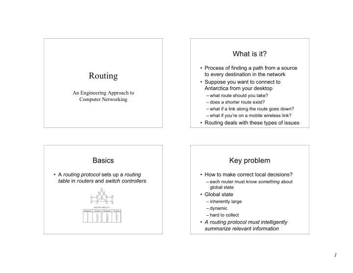
Basics

A routing protocol sets up a routing

table in routers and switch controllers

Key problem

How to make correct local decisions?

– each router must know something about global state

Global state

– inherently large – dynamic – hard to collect

A routing protocol must intelligently

summarize relevant information

SLIDE 2

2

Requirements

Minimize routing table space

– fast to look up – less to exchange

Minimize number and frequency of control

messages

Robustness: avoid

– black holes – loops – oscillations

Use optimal path

Choices

Centralized vs. distributed routing

– centralized is simpler, but prone to failure and congestion

Source-based vs. hop-by-hop

– how much is in packet header? – Intermediate: loose source route

Stochastic vs. deterministic

– stochastic spreads load, avoiding oscillations, but misorders

Single vs. multiple path

– primary and alternative paths (compare with stochastic)

State-dependent vs. state-independent

– do routes depend on current network state (e.g. delay)

Outline

Routing in telephone networks
Distance-vector routing
Link-state routing
Choosing link costs
Hierarchical routing
Internet routing protocols
Routing within a broadcast LAN
Multicast routing
Routing with policy constraints
Routing for mobile hosts

Telephone network topology

3-level hierarchy, with a fully-connected core
AT&T: 135 core switches with nearly 5 million

circuits

LECs may connect to multiple cores

SLIDE 3

3

Routing algorithm

If endpoints are within same CO, directly

connect

If call is between COs in same LEC, use one-

hop path between COs

Otherwise send call to one of the cores
Only major decision is at toll switch

– one-hop or two-hop path to the destination toll switch – (why don’t we need longer paths?)

Essence of problem

– which two-hop path to use if one-hop path is full

Features of telephone network routing

Stable load

– can predict pairwise load throughout the day – can choose optimal routes in advance

Extremely reliable switches

– downtime is less than a few minutes per year – can assume that a chosen route is available – can’t do this in the Internet

Single organization controls entire core

– can collect global statistics and implement global changes

Very highly connected network
Connections require resources (but all need

the same)

Statistics

Posson call arrival (independence

assumption)

Exponential call “holding” time (length!)
Goal:- Minimise Call “Blocking” (aka

“loss”) Probability subject to minimise cost of network

The cost of simplicity

Simplicity of routing a historical necessity
But requires

– reliability in every component – logically fully-connected core

Can we build an alternative that has same

features as the telephone network, but is cheaper because it uses more sophisticated routing?

– Yes: that is one of the motivations for ATM – But 80% of the cost is in the local loop

not affected by changes in core routing

– Moreover, many of the software systems assume topology

too expensive to change them

SLIDE 4

4

Dynamic nonhierarchical routing (DNHR)

Simplest core routing protocol

– accept call if one-hop path is available, else drop

DNHR

– divides day into around 10-periods – in each period, each toll switch is assigned a primary one-hop path and a list of alternatives – can overflow to alternative if needed – drop only if all alternate paths are busy

crankback
Problems

– does not work well if actual traffic differs from prediction

Metastability

Burst of activity can cause network to enter

metastable state

– high blocking probability even with a low load

Removed by trunk reservation

– prevents spilled traffic from taking over direct path

Trunk status map routing (TSMR)

DNHR measures traffic once a week
TSMR updates measurements once an

hour or so

– only if it changes “significantly”

List of alternative paths is more up to

date

Real-time network routing

No centralized control

– Each toll switch maintains a list of lightly loaded links – Intersection of source and destination lists gives set of lightly loaded paths

Example

– At A, list is C, D, E => links AC, AD, AE lightly loaded – At B, list is D, F, G => links BD, BF, BG lightly loaded – A asks B for its list – Intersection = D => AD and BD lightly loaded => ADB lightly loaded => it is a good alternative path

Very effective in practice: only about a couple
f calls blocked in core out of about 250

million calls attempted every day

SLIDE 5

5

November 2001 Dynamic Alternative Routing 17

D Dynamic

ynamic

A

Alternative

lternative

R

Routing

uting

Very simple idea, but can be shown to provide optimal routes at very low complexity…

November 2001 Dynamic Alternative Routing 18

Underlying Network Properties Underlying Network Properties

Fully connected network
Underlying network is a trunk network
Relatively small number of nodes
In 1986, the trunk network of British Telecom had
nly 50 nodes
Any algorithm with polynomial running time works

fine

Stochastic traffic
Low variance when the link is nearly saturated

November 2001 Dynamic Alternative Routing 19

Dynamic Alternative Routing Dynamic Alternative Routing

Proposed by F.P. Kelly, R.

Gibbens at British Telecom (well, Cambridge, Really:)

Whenever the link (i, j) is

saturated, use an alternative node (tandem)

Q. How to choose tandem?

i j Ci,j k

November 2001 Dynamic Alternative Routing 20

Fixed Tandem Fixed Tandem

For any pair of nodes (i, j) we assign a fixed

node k as tandem

Needs careful traffic analysis and

reprogramming

Inflexible during breakdowns and unexpected

traffic at tandem

SLIDE 6

6

November 2001 Dynamic Alternative Routing 21

Sticky Random Tandem Sticky Random Tandem

If there is no free circuit along (i, j), a new call is

routed through a randomly chosen tandem k

k is the tandem as long as it does not fail
If k fails for a call, the call is lost and a new

tandem is selected

November 2001 Dynamic Alternative Routing 22

Sticky Random Tandem Sticky Random Tandem

Decentralized and flexible
No fancy pre-analysis of traffic required
Most of the time friendly tandems are used:
pk(i, j): proportion of calls between i and j which go

through k

qk(i, j): proportion of calls that are blocked

pa(i, j)qa(i, j) = pb(i, j)qb(i, j)

We may assign different frequencies to different

tandems

November 2001 Dynamic Alternative Routing 23

Trunk Reservation Trunk Reservation

Unselfishness towards one’s friends

is good up to a point!!!

We need to penalize two link calls,

at least when the lines are very busy! A tandem k accepts to forward calls if it has free capacity more than R

i j k

November 2001 Dynamic Alternative Routing 24

Trunk Reservation Trunk Reservation

SLIDE 7

7

November 2001 Dynamic Alternative Routing 25

Bounds: Bounds: Erlang Erlang’ ’s s Bound Bound

A node connected to C circuits
Arrival: Poisson with mean v
The expected value of blocking:

1 0 !

! ) , (

=
=

C i i c

i v C v C v E

November 2001 Dynamic Alternative Routing 26

Max-flow Bound Max-flow Bound

Capacity of (i, j): Cij
Mean load on (i, j):

vij

where f is:

i j Cij

)) ( ( ) ( t v f t n E

j i ij

<
<
+

j i j i k ikj ij

x x

,

max

k

November 2001 Dynamic Alternative Routing 27

Trunk Reservation Trunk Reservation

November 2001 Dynamic Alternative Routing 28

Traffic, Capacity Mismatch Traffic, Capacity Mismatch

Traffic > Capacity for

some links

Can we always find a

feasible set of tandems?

Red links: saturated links
White links: not saturated
Good triangle: one red,

two white links

SLIDE 8

8

November 2001 Dynamic Alternative Routing 29

Greedy Algorithm Greedy Algorithm

T1 T2 Tk+1

a. No red links
b. Red link and a

good triangle

Add good

triangle to the list

c. Red link and no

good triangle Success! Success! Tk Fail

November 2001 Dynamic Alternative Routing 30

T1 T2 Tk+1

a. No red links
b. Red link and a

good triangle

Add good

triangle to the list

c. Red link and no

good triangle Success! Success! Tk Fail

For any p < 1/3, the greedy algorithm is successful with probability approaching 1.

Greedy Algorithm Greedy Algorithm

November 2001 Dynamic Alternative Routing 31

Extensions to DAR Extensions to DAR

n-link paths
Too much resources consumed, little benefit
Multiple alternatives
M attempts before rejecting a call
Least-busy alternative
Repacking
A call in progress can be rerouted

November 2001 Dynamic Alternative Routing 32

Comparison of Extensions Comparison of Extensions

SLIDE 9

9

Features of Internet Routing

Packets, not circuits (

– E.g. timescales can be much shorter

Topology complicated/heterogeneous
Many (10,000 ++) providers
Traffic sources bursty
Traffic matrix unpredictable

– E.g. Not distance constrained

Goal: maximise throughput, subject to min

delay and cost (and energy?)

Internet Routing Model

2 key features:

– Dynamic routing – Intra- and Inter-AS routing, AS = locus of admin control

Internet organized as “autonomous systems” (AS).

– AS is internally connected

Interior Gateway Protocols (IGPs) within AS.

– Eg: RIP, OSPF, HELLO

Exterior Gateway Protocols (EGPs) for AS to AS routing.

– Eg: EGP, BGP-4

Requirements for Intra-AS Routing

Should scale for the size of an AS.

– Low end: 10s of routers (small enterprise) – High end: 1000s of routers (large ISP)

Different requirements on routing convergence after

topology changes

– Low end: can tolerate some connectivity disruptions – High end: fast convergence essential to business (making money

n transport)
Operational/Admin/Management (OAM) Complexity

– Low end: simple, self-configuring – High end: Self-configuring, but operator hooks for control

Traffic engineering capabilities: high end only

Requirements for Inter-AS Routing

Should scale for the size of the global Internet.

– Focus on reachability, not optimality – Use address aggregation techniques to minimize core routing table sizes and associated control traffic – At the same time, it should allow flexibility in topological structure (eg: don’t restrict to trees etc)

Allow policy-based routing between autonomous systems

– Policy refers to arbitrary preference among a menu of available

ptions (based upon options’ attributes)

– In the case of routing, options include advertised AS-level routes to address prefixes – Fully distributed routing (as opposed to a signaled approach) is the only possibility. – Extensible to meet the demands for newer policies.

SLIDE 10

10

Intra-AS and Inter-AS routing

inter-AS, intra-AS routing in gateway A.c network layer link layer physical layer

a b b a a C A B d

Gateways:

perform inter-AS

routing amongst themselves

perform intra-AS

routers with other routers in their AS A.c A.a C.b B.a c b c

Intra-AS and Inter-AS routing: Example

Host h2 a b b a a C A B d c A.a A.c C.b B.a c b Host h1 Intra-AS routing within AS A Inter-AS routing between A and B Intra-AS routing within AS B

Basic Dynamic Routing Methods

Source-based: source gets a map of the network,

– source finds route, and either – signals the route-setup (eg: ATM approach) – encodes the route into packets (inefficient)

Link state routing: per-link information

– Get map of network (in terms of link states) at all nodes and find next-hops locally. – Maps consistent => next-hops consistent

Distance vector: per-node information

– At every node, set up distance signposts to destination nodes (a vector) – Setup this by peeking at neighbors’ signposts.

 Routing vs Forwarding  Forwarding table vs Forwarding in simple topologies  Routers vs Bridges: review  Routing Problem  Telephony vs Internet Routing  Source-based vs Fully distributed Routing  Distance vector vs Link state routing

 Bellman Ford and Dijkstra Algorithms

 Addressing and Routing: Scalability

Where are we?

SLIDE 11

11

DV & LS: consistency criterion

The subset of a shortest path is also the shortest

path between the two intermediate nodes.

Corollary:

– If the shortest path from node i to node j, with distance D(i,j) passes through neighbor k, with link cost c(i,k), then:

D(i,j) = c(i,k) + D(k,j)

i k j c ( i , k ) D ( k , j )

Distance Vector

DV = Set (vector) of Signposts, one for each destination

Distance Vector (DV) Approach

Consistency Condition: D(i,j) = c(i,k) + D(k,j)

The DV (Bellman-Ford) algorithm evaluates this

recursion iteratively.

– In the mth iteration, the consistency criterion holds, assuming that each node sees all nodes and links m- hops (or smaller) away from it (i.e. an m-hop view)

A E D C B

7 8 1 2 1 2

Example network

A E D C B

7 8 1 2 1

A’s 2-hop view (After 2nd Iteration)

A E B

7 1

A’s 1-hop view (After 1st iteration)

Distance Vector (DV)…

Initial distance values (iteration 1):

– D(i,i) = 0 ; – D(i,k) = c(i,k) if k is a neighbor (i.e. k is one-hop away); and – D(i,j) = INFINITY for all other non-neighbors j.

Note that the set of values D(i,*) is a distance

vector at node i.

The algorithm also maintains a next-hop

value (forwarding table) for every destination j, initialized as:

– next-hop(i) = i; – next-hop(k) = k if k is a neighbor, and – next-hop(j) = UNKNOWN if j is a non-neighbor.

SLIDE 12

12

Distance Vector (DV)…

After every iteration each node i exchanges

its distance vectors D(i,*) with its immediate neighbors.

For any neighbor k, if c(i,k) + D(k,j) < D(i,j),

then:

– D(i,j) = c(i,k) + D(k,j) – next-hop(j) = k

After each iteration, the consistency criterion

is met

– After m iterations, each node knows the shortest path possible to any other node which is m hops

r less.

– I.e. each node has an m-hop view of the network. – The algorithm converges (self-terminating) in O(d) iterations: d is the maximum diameter of the network.

Distance Vector (DV) Example

A’s distance vector D(A,*):

– After Iteration 1 is: [0, 7, INFINITY, INFINITY, 1] – After Iteration 2 is: [0, 7, 8, 3, 1] – After Iteration 3 is: [0, 7, 5, 3, 1] – After Iteration 4 is: [0, 6, 5, 3, 1]

A E D C B

7 8 1 2 1 2

Example network

A E D C B

7 8 1 2 1

A’s 2-hop view (After 2nd Iteration)

A E B

7 1

A’s 1-hop view (After 1st iteration)

Distance Vector: link cost changes

Link cost changes: node detects local link cost change updates distance table if cost change in least cost path, notify neighbors

X Z

1 4 50

Y

1

algorithm terminates

“good news travels fast” [ 2 1 0] [ 5 1 0] [ 5 1 0] DV(Z) [ 1 0 1] [ 1 0 1] [ 4 0 1] DV(Y)

Iter. 2
Iter. 1

Time 0

Distance Vector: link cost changes

Link cost changes: good news travels fast bad news travels slow - “count to infinity” problem!

X Z

1 4 50

Y

60

algo goes

n!

[ 7 1 0] [ 8 0 1] Iter 3 [ 9 1 0] [ 8 0 1] Iter 4 [ 7 1 0] [ 5 1 0] [ 5 1 0] DV(Z) [ 6 0 1] [ 6 0 1] [ 4 0 1] DV(Y) Iter 2 Iter 1 Time 0

SLIDE 13

13

Distance Vector: poisoned reverse

If Z routes through Y to get to X : Z tells Y its (Z’s) distance to X is infinite (so Y won’t route to X via Z) At Time 0, DV(Z) as seen by Y is [INF INF 0], not [5 1 0] !

X Z

1 4 50

Y

60

algorithm terminates

[ 7 1 0] [ 51 0 1] Iter 3 [ 50 1 0] [ 5 1 0] [ 5 1 0] DV(Z) [ 60 0 1] [ 60 0 1] [ 4 0 1] DV(Y) Iter 2 Iter 1 Time 0

Link State (LS) Approach

The link state (Dijkstra) approach is iterative, but it pivots

around destinations j, and their predecessors k = p(j)

– Observe that an alternative version of the consistency condition holds for this case: D(i,j) = D(i,k) + c(k,j)

Each node i collects all link states c(*,*) first and runs the

complete Dijkstra algorithm locally. i k j c ( k , j ) D(i,k)

Link State (LS) Approach…

After each iteration, the algorithm finds a new destination

node j and a shortest path to it.

After m iterations the algorithm has explored paths, which

are m hops or smaller from node i.

– It has an m-hop view of the network just like the distance-vector approach

The Dijkstra algorithm at node i maintains two sets:

– set N that contains nodes to which the shortest paths have been found so far, and – set M that contains all other nodes. – For all nodes k, two values are maintained:

D(i,k): current value of distance from i to k.
p(k): the predecessor node to k on the shortest known path from i

Dijkstra: Initialization

Initialization:

– D(i,i) = 0 and p(i) = i; – D(i,k) = c(i,k) and p(k) = i if k is a neighbor of I – D(i,k) = INFINITY and p(k) = UNKNOWN if k is not a neighbor of I – Set N = { i }, and next-hop (i) = I – Set M = { j | j is not i}

Initially set N has only the node i and set M has the rest
f the nodes.
At the end of the algorithm, the set N contains all the

nodes, and set M is empty

SLIDE 14

14

Dijkstra: Iteration

In each iteration, a new node j is moved from set M into

the set N.

– Node j has the minimum distance among all current nodes in M, i.e. D(i,j) = min {l ε M} D(i,l). – If multiple nodes have the same minimum distance, any one of them is chosen as j. – Next-hop(j) = the neighbor of i on the shortest path

Next-hop(j) = next-hop(p(j)) if p(j) is not i
Next-hop(j) = j

if p(j) = i

– Now, in addition, the distance values of any neighbor k of j in set M is reset as:

If D(i,k) < D(i,j) + c(j,k), then

D(i,k) = D(i,j) + c(j,k), and p(k) = j.

This operation is called “relaxing” the edges of node j.

Dijkstra’s algorithm: example

Step 1 2 3 4 5 set N A AD ADE ADEB ADEBC ADEBCF D(B),p(B) 2,A 2,A 2,A D(C),p(C) 5,A 4,D 3,E 3,E D(D),p(D) 1,A D(E),p(E) infinity 2,D D(F),p(F) infinity infinity 4,E 4,E 4,E A E D C B F

2 2 1 3 1 1 2 5 3 5

The shortest-paths spanning tree rooted at A is called an SPF-tree

Misc Issues: Transient Loops

With consistent

LSDBs, all nodes compute consistent loop-free paths

Limited by Dijkstra

computation

verhead, space

requirements

Can still have

transient loops

A B C D 1 3 5 2 1

Packet from CA may loop around BDC if B knows about failure and C & D do not X

Dijkstra’s algorithm, discussion

Algorithm complexity: n nodes  each iteration: need to check all nodes, w, not in N  n*(n+1)/2 comparisons: O(n**2)  more efficient implementations possible: O(nlogn) Oscillations possible:  e.g., link cost = amount of carried traffic A D C B

1 1+e e e 1 1

A D C B

2+e 1+e 1

A D C B

2+e 1+e 1 0 0

A D C B

2+e e 1+e 1

initially … recompute routing … recompute … recompute

SLIDE 15

15

Misc: How to assign the Cost Metric?

Choice of link cost defines traffic load

– Low cost = high probability link belongs to SPT and will attract traffic

Tradeoff: convergence vs load distribution

– Avoid oscillations – Achieve good network utilization

Static metrics (weighted hop count)

– Does not take traffic load (demand) into account.

Dynamic metrics (cost based upon queue or delay etc)

– Highly oscillatory, very hard to dampen (DARPAnet experience)

Quasi-static metric:

– Reassign static metrics based upon overall network load (demand matrix), assumed to be quasi-stationary

Misc: Incremental SPF

Dijkstra algorithm is invoked whenever a new

LS update is received.

– Most of the time, the change to the SPT is minimal, or even nothing

If the node has visibility to a large number of

prefixes, then it may see large number of updates.

– Flooding bugs further exacerbate the problem – Solution: incremental SPF algorithms which use knowledge of current map and SPT, and process the delta change with lower computational complexity compared to Dijkstra – Avg case: O(logn) v. to O(nlogn) for Dijkstra

Ref: Alaettinoglu, Jacobson, Yu, “Towards Milli-Second IGP Convergence,” Internet Draft.

Topology information is

flooded within the routing domain

Best end-to-end paths are

computed locally at each router.

Best end-to-end paths

determine next-hops.

Based on minimizing some

notion of distance

Works only if policy is shared

and uniform

Examples: OSPF, IS-IS
Each router knows little

about network topology

Only best next-hops are

chosen by each router for each destination network.

Best end-to-end paths result

from composition of all next- hop choices

Does not require any notion
f distance
Does not require uniform

policies at all routers

Examples: RIP, BGP

Link State Vectoring

Summary: Distributed Routing Techniques

Link state: topology dissemination

A router describes its neighbors with a link

state packet (LSP)

Use controlled flooding to distribute this

everywhere

– store an LSP in an LSP database – if new, forward to every interface other than incoming one – a network with E edges will copy at most 2E times

SLIDE 16

16

Sequence numbers

How do we know an LSP is new?
Use a sequence number in LSP header
Greater sequence number is newer
What if sequence number wraps around?

– smaller sequence number is now newer! – (hint: use a large sequence space)

On boot up, what should be the initial

sequence number?

– have to somehow purge old LSPs – two solutions

aging
lollipop sequence space

Aging

Creator of LSP puts timeout value in the

header

Router removes LSP when it times out

– also floods this information to the rest of the network (why?)

So, on booting, router just has to wait for its
ld LSPs to be purged
But what age to choose?

– if too small

purged before fully flooded (why?)
needs frequent updates

– if too large

router waits idle for a long time on rebooting

A better solution

Need a unique start sequence number
a is older than b if:

– a < 0 and a < b – a > o, a < b, and b-a < N/4 – a > 0, b > 0, a > b, and a-b > N/4

More on lollipops

If a router gets an older LSP, it tells the

sender about the newer LSP

So, newly booted router quickly finds
ut its most recent sequence number
It jumps to one more than that
-N/2 is a trigger to evoke a response

from community memory

SLIDE 17

17

Recovering from a partition

On partition, LSP databases can get out of

synch

Databases described by database descriptor

records

Routers on each side of a newly restored link

talk to each other to update databases (determine missing and out-of-date LSPs)

Router failure

How to detect?

– HELLO protocol

HELLO packet may be corrupted

– so age anyway – on a timeout, flood the information

Securing LSP databases

LSP databases must be consistent to

avoid routing loops

Malicious agent may inject spurious

LSPs

Routers must actively protect their

databases

– checksum LSPs – ack LSP exchanges – passwords

Outline

Routing in telephone networks
Distance-vector routing
Link-state routing
Choosing link costs
Hierarchical routing
Internet routing protocols
Routing within a broadcast LAN
Multicast routing
Routing with policy constraints
Routing for mobile hosts

SLIDE 18

18

Choosing link costs

Shortest path uses link costs
Can use either static of dynamic costs
In both cases: cost determine amount of

traffic on the link

– lower the cost, more the expected traffic – if dynamic cost depends on load, can have

scillations (why?)

Static metrics

Simplest: set all link costs to 1 => min

hop routing

– but 28.8 modem link is not the same as a T3!

Give links weight proportional to

capacity

Dynamic metrics

A first cut (ARPAnet original)
Cost proportional to length of router queue

– independent of link capacity

Many problems when network is loaded

– queue length averaged over a small time => transient spikes caused major rerouting – wide dynamic range => network completely ignored paths with high costs – queue length assumed to predict future loads =>

pposite is true (why?)

– no restriction on successively reported costs =>

scillations

– all tables computed simultaneously => low cost link flooded

Modified metrics

– queue length averaged

ver a small time

– wide dynamic range queue – queue length assumed to predict future loads – no restriction on successively reported costs – all tables computed simultaneously – queue length averaged

ver a longer time

– dynamic range restricted – cost also depends on intrinsic link capacity – restriction on successively reported costs – attempt to stagger table computation

SLIDE 19

19

Routing dynamics Outline

Routing in telephone networks
Distance-vector routing
Link-state routing
Choosing link costs
Hierarchical routing
Internet routing protocols
Routing within a broadcast LAN
Multicast routing
Routing with policy constraints
Routing for mobile hosts

Hierarchical routing

Large networks need large routing tables

– more computation to find shortest paths – more bandwidth wasted on exchanging DVs and LSPs

Solution:

– hierarchical routing

Key idea

– divide network into a set of domains – gateways connect domains – computers within domain unaware of outside computers – gateways know only about other gateways

Example

Features

– only a few routers in each level – not a strict hierarchy – gateways participate in multiple routing protocols – non-aggregable routers increase core table space

SLIDE 20

20

Hierarchy in the Internet

Three-level hierarchy in addresses

– network number – subnet number/more specific prefix – host number

Core advertises routes only to networks, not

to subnets

– e.g. 135.104.*, 192.20.225.*

Even so, about 80,000 networks in core

routers (1996)

Gateways talk to backbone to find best next-

hop to every other network in the Internet

External and summary records

If a domain has multiple gateways

– external records tell hosts in a domain which one to pick to reach a host in an external domain

e.g allows 6.4.0.0 to discover shortest path to 5.* is

through 6.0.0.0

– summary records tell backbone which gateway to use to reach an internal node

e.g. allows 5.0.0.0 to discover shortest path to 6.4.0.0 is

through 6.0.0.0

External and summary records contain

distance from gateway to external or internal node

– unifies distance vector and link state algorithms

Interior and exterior protocols

Internet has three levels of routing

– highest is at backbone level, connecting autonomous systems (AS) – next level is within AS – lowest is within a LAN

Protocol between AS gateways: exterior

gateway protocol

Protocol within AS: interior gateway

protocol

Exterior gateway protocol

Between untrusted routers

– mutually suspicious

Must tell a border gateway who can be

trusted and what paths are allowed

Transit over backdoors is a problem

SLIDE 21

21

Interior protocols

Much easier to implement
Typically partition an AS into areas
Exterior and summary records used

between areas

Issues in interconnection

May use different schemes (DV vs. LS)
Cost metrics may differ
Need to:

– convert from one scheme to another (how?) – use the lowest common denominator for costs – manually intervene if necessary

Outline

Routing in telephone networks
Distance-vector routing
Link-state routing
Choosing link costs
Hierarchical routing
Internet routing protocols
Routing within a broadcast LAN
Multicast routing
Routing with policy constraints
Routing for mobile hosts

Common routing protocols

Interior

– RIP – OSPF

Exterior

– EGP – BGP

ATM

– PNNI

SLIDE 22

22

RIP

Distance vector
Cost metric is hop count
Infinity = 16
Exchange distance vectors every 30 s
Split horizon
Useful for small subnets

– easy to install

OSPF

Link-state
Uses areas to route packets

hierarchically within AS

Complex

– LSP databases to be protected

Uses designated routers to reduce

number of endpoints

EGP

Original exterior gateway protocol
Distance-vector
Costs are either 128 (reachable) or 255

(unreachable) => reachability protocol => backbone must be loop free (why?)

Allows administrators to pick neighbors

to peer with

Allows backdoors (by setting backdoor

cost < 128)

BGP

Path-vector

– distance vector annotated with entire path – also with policy attributes – guaranteed loop-free

Can use non-tree backbone topologies
Uses TCP to disseminate DVs

– reliable – but subject to TCP flow control

Policies are complex to set up

SLIDE 23

23

PNNI (ATM/cell switched)

Link-state
Many levels of hierarchy

– Switch controllers at each level form a peer group – Group has a group leader – Leaders are members of the next higher level group – Leaders summarize information about group to tell higher level peers – All records received by leader are flooded to lower level

LSPs can be annotated with per-link QoS

metrics

Switch controller uses this to compute source

routes for call-setup packets

Outline

Routing in telephone networks
Distance-vector routing
Link-state routing
Choosing link costs
Hierarchical routing
Internet routing protocols
Routing within a broadcast LAN
Multicast routing
Routing with policy constraints
Routing for mobile hosts

Routing within a broadcast LAN

What happens at an endpoint?
On a point-to-point link, no problem
On a broadcast LAN

– is packet meant for destination within the LAN? – if so, what is the datalink address ? – if not, which router on the LAN to pick? – what is the router’s datalink address?

Internet solution

All hosts on the LAN have the same subnet

address

So, easy to determine if destination is on the

same LAN

Destination’s datalink address determined

using ARP

– broadcast a request – owner of IP address replies

To discover routers

– routers periodically sends router advertisements

with preference level and time to live

– pick most preferred router – delete overage records – can also force routers to reply with solicitation message

SLIDE 24

24

Redirection

How to pick the best router?
Send message to arbitrary router
If that router’s next hop is another router
n the same LAN, host gets a redirect

message

It uses this for subsequent messages

Outline

Routing in telephone networks
Distance-vector routing
Link-state routing
Choosing link costs
Hierarchical routing
Internet routing protocols
Routing within a broadcast LAN
Multicast routing
Routing with policy constraints
Routing for mobile hosts

Multicast routing

Unicast: single source sends to a single

destination

Multicast: hosts are part of a multicast group

– packet sent by any member of a group are received by all

Useful for

– multiparty videoconference – distance learning – resource location

Multicast group

Associates a set of senders and receivers with

each other

– but independent of them – created either when a sender starts sending from a group – or a receiver expresses interest in receiving – even if no one else is there!

Sender does not need to know receivers’ identities

– rendezvous point

SLIDE 25

25

Addressing

Multicast group in the Internet has its own

Class D address

– looks like a host address, but isn’t

Senders send to the address
Receivers anywhere in the world request

packets from that address

“Magic” is in associating the two: dynamic

directory service

Four problems

– which groups are currently active – how to express interest in joining a group – discovering the set of receivers in a group – delivering data to members of a group

Expanding ring search

A way to use multicast groups for resource

discovery

Routers decrement TTL when forwarding
Sender sets TTL and multicasts

– reaches all receivers <= TTL hops away

Discovers local resources first
Since heavily loaded servers can keep quiet,

automatically distributes load

Multicast flavors

Unicast: point to point
Multicast:

– point to multipoint – multipoint to multipoint

Can simulate point to multipoint by a set of

point to point unicasts

Can simulate multipoint to multipoint by a set
f point to multipoint multicasts
The difference is efficiency

Example

Suppose A wants to talk to B, G, H, I, B to A,

G, H, I

With unicast, 4 messages sent from each

source

– links AC, BC carry a packet in triplicate

With point to multipoint multicast, 1 message

sent from each source

– but requires establishment of two separate multicast groups

With multipoint to multipoint multicast, 1

message sent from each source,

SLIDE 26

26

Shortest path tree

Ideally, want to send exactly one multicast

packet per link

– forms a multicast tree rooted at sender

Optimal multicast tree provides shortest path

from sender to every receiver

– shortest-path tree rooted at sender

Issues in wide-area multicast

Difficult because

– sources may join and leave dynamically

need to dynamically update shortest-path tree

– leaves of tree are often members of broadcast LAN

would like to exploit LAN broadcast capability

– would like a receiver to join or leave without explicitly notifying sender

otherwise it will not scale

Multicast in a broadcast LAN

Wide area multicast can exploit a LAN’s

broadcast capability

E.g. Ethernet will multicast all packets with

multicast bit set on destination address

Two problems:

– what multicast MAC address corresponds to a given Class D IP address? – does the LAN have contain any members for a given group (why do we need to know this?)

Class D to MAC translation

Multiple Class D addresses map to the same

MAC address

Well-known translation algorithm => no need

for a translation table

01 00 5E 23 bits copied from IP address IEEE 802 MAC Address Class D IP address Ignored ‘1110’ = Class D indication Multicast bit Reserved bit

SLIDE 27

27

Group Management Protocol

Detects if a LAN has any members for a particular

group

– If no members, then we can prune the shortest path tree for that group by telling parent

Router periodically broadcasts a query message
Hosts reply with the list of groups they are interested

in

To suppress traffic

– reply after random timeout – broadcast reply – if someone else has expressed interest in a group, drop

ut
To receive multicast packets:

– translate from class D to MAC and configure adapter

Wide area multicast

Assume

– each endpoint is a router – a router can use IGMP to discover all the members in its LAN that want to subscribe to each multicast group

Goal

– distribute packets coming from any sender directed to a given group to all routers on the path to a group member

Simplest solution

Flood packets from a source to entire network
If a router has not seen a packet before,

forward it to all interfaces except the incoming

ne
Pros

– simple – always works!

Cons

– routers receive duplicate packets – detecting that a packet is a duplicate requires storage, which can be expensive for long multicast sessions

A clever solution

Reverse path forwarding
Rule

– forward packet from S to all interfaces if and only if packet arrives on the interface that corresponds to the shortest path to S – no need to remember past packets – C need not forward packet received from D

SLIDE 28

28

Cleverer

Don’t send a packet downstream if you are

not on the shortest path from the downstream router to the source

C need not forward packet from A to E
Potential confusion if downstream router has

a choice of shortest paths to source (see figure on previous slide)

Pruning

RPF does not completely eliminate

unnecessary transmissions

B and C get packets even though they do not

need it

Pruning => router tells parent in tree to stop

forwarding

Can be associated either with a multicast

group or with a source and group

Rejoining

What if host on C’s LAN wants to receive

messages from A after a previous prune by C?

– IGMP lets C know of host’s interest – C can send a join(group, A) message to B, which propagates it to A – or, periodically flood a message; C refrains from pruning

A problem

Reverse path forwarding requires a

router to know shortest path to a source

– known from routing table

Doesn’t work if some routers do not

support multicast

– virtual links between multicast-capable routers – shortest path to A from E is not C, but F

SLIDE 29

29

A problem (contd.)

Two problems

– how to build virtual links – how to construct routing table for a network with virtual links

Tunnels

Why do we need them?
Consider packet sent from A to F via

multicast-incapable D

If packet’s destination is Class D, D drops it
If destination is F’s address, F doesn’t know

multicast address!

So, put packet destination as F, but carry

multicast address internally

Encapsulate IP in IP => set protocol type to

IP-in-IP

Multicast routing protocol

Interface on “shortest path” to source

depends on whether path is real or virtual

Shortest path from E to A is not through C,

but F

– so packets from F will be flooded, but not from C

Need to discover shortest paths only taking

multicast-capable routers into account

– DVMRP

DVMRP

Distance-vector Multicast routing protocol
Very similar to RIP

– distance vector – hop count metric

Used in conjunction with

– flood-and-prune (to determine memberships)

prunes store per-source and per-group information

– reverse-path forwarding (to decide where to forward a packet) – explicit join messages to reduce join latency (but no source info, so still need flooding)

SLIDE 30

30

MOSPF

Multicast extension to OSPF
Routers flood group membership information

with LSPs

Each router independently computes

shortest-path tree that only includes multicast-capable routers

– no need to flood and prune

Complex

– interactions with external and summary records – need storage per group per link – need to compute shortest path tree per source and group

Core-based trees

Problems with DVMRP-oriented approach

– need to periodically flood and prune to determine group members – need to source per-source and per-group prune records at each router

Key idea with core-based tree

– coordinate multicast with a core router – host sends a join request to core router – routers along path mark incoming interface for forwarding

Example

Pros

– routers not part of a group are not involved in pruning – explicit join/leave makes membership changes faster – router needs to store only one record per group

Cons

– all multicast traffic traverses core, which is a bottleneck – traffic travels on non-optimal paths

Protocol independent multicast (PIM)

Tries to bring together best aspects of CBT

and DVMRP

Choose different strategies depending on

whether multicast tree is dense or sparse

– flood and prune good for dense groups

only need a few prunes
CBT needs explicit join per source/group

– CBT good for sparse groups

Dense mode PIM == DVMRP
Sparse mode PIM is similar to CBT

– but receivers can switch from CBT to a shortest- path tree

SLIDE 31

31

PIM (contd.)

In CBT, E must send to core
In PIM, B discovers shorter path to E (by

looking at unicast routing table)

– sends join message directly to E – sends prune message towards core

Core no longer bottleneck
Survives failure of core

More on core

Renamed a rendezvous point

– because it no longer carries all the traffic like a CBT core

Rendezvous points periodically send “I am

alive” messages downstream

Leaf routers set timer on receipt
If timer goes off, send a join request to

alternative rendezvous point

Problems

– how to decide whether to use dense or sparse mode? – how to determine “best” rendezvous point?

Outline

Routing in telephone networks
Distance-vector routing
Link-state routing
Choosing link costs
Hierarchical routing
Internet routing protocols
Routing within a broadcast LAN
Multicast routing
Routing with policy constraints
Routing for mobile hosts

Routing vs. policy routing

In standard routing, a packet is forwarded on

the ‘best’ path to destination

– choice depends on load and link status

With policy routing, routes are chosen

depending on policy directives regarding things like

– source and destination address – transit domains – quality of service – time of day – charging and accounting

The general problem is still open

– fine balance between correctness and information hiding

SLIDE 32

32

Multiple metrics

Simplest approach to policy routing
Advertise multiple costs per link
Routers construct multiple shortest path

trees

Problems with multiple metrics

All routers must use the same rule in

computing paths

Remote routers may misinterpret policy

– source routing may solve this – but introduces other problems (what?)

Provider selection

Another simple approach
Assume that a single service provider

provides almost all the path from source to destination

– e.g. AT&T or MCI

Then, choose policy simply by choosing

provider

– this could be dynamic (agents!)

In Internet, can use a loose source route

through service provider’s access point

Or, multiple addresses/names per host

Crankback

Consider computing routes with QoS

guarantees

Router returns packet if no next hop with

sufficient QoS can be found

In ATM networks (PNNI) used for the call-

setup packet

In Internet, may need to be done for _every_

packet!

– Will it work?

SLIDE 33

33

Outline

Routing in telephone networks
Distance-vector routing
Link-state routing
Choosing link costs
Hierarchical routing
Internet routing protocols
Routing within a broadcast LAN
Multicast routing
Routing with policy constraints
Routing for mobile hosts

Mobile routing

How to find a mobile host?
Two sub-problems

– location (where is the host?) – routing (how to get packets to it?)

We will study mobile routing in the

Internet and in the telephone network

Mobile cellular routing

Each cell phone has a global ID that it tells

remote MTSO when turned on (using slotted ALOHA up channel)

Remote MTSO tells home MTSO
To phone: call forwarded to remote MTSO to

closest base

From phone: call forwarded to home MTSO

from closest base

Mobile routing in the Internet

Very similar to mobile telephony

– but outgoing traffic does not go through home – and need to use tunnels to forward data

Use registration packets instead of slotted

ALOHA

– passed on to home address agent

Old care-of-agent forwards packets to new

care-of-agent until home address agent learns of change

SLIDE 34

34

Problems

Security

– mobile and home address agent share a common secret – checked before forwarding packets to COA

Loops