Routing Mechanisms for Interconnection Networks Routing a message - - PowerPoint PPT Presentation

routing mechanisms for interconnection networks
SMART_READER_LITE
LIVE PREVIEW

Routing Mechanisms for Interconnection Networks Routing a message - - PowerPoint PPT Presentation

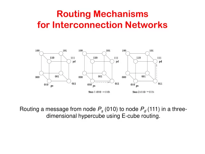
Routing Mechanisms for Interconnection Networks Routing a message from node P s (010) to node P d (111) in a three- dimensional hypercube using E-cube routing. Mapping Techniques for Graphs Often, we need to embed a known communication


slide-1
SLIDE 1

Routing Mechanisms for Interconnection Networks

Routing a message from node Ps (010) to node Pd (111) in a three- dimensional hypercube using E-cube routing.

slide-2
SLIDE 2

Mapping Techniques for Graphs

  • Often, we need to embed a known communication

pattern into a given interconnection topology.

  • We may have an algorithm designed for one network,

which we are porting to another topology. For these reasons, it is useful to understand mapping between graphs.

slide-3
SLIDE 3

Mapping Techniques for Graphs: Metrics

  • When mapping a graph G(V,E) into G’(V’,E’), the

following metrics are important:

  • The maximum number of edges mapped onto any edge

in E’ is called the congestion of the mapping.

  • The maximum number of links in E’ that any edge in E is
  • mapped onto is called the dilation of the mapping.
  • The ratio of the number of nodes in the set V’ to that in

set V is called the expansion of the mapping.

slide-4
SLIDE 4

Embedding a Linear Array into a Hypercube

  • A linear array (or a ring) composed of 2d nodes (labeled

0 through 2d − 1) can be embedded into a d-dimensional hypercube by mapping node i of the linear array onto node

  • G(i, d) of the hypercube. The function G(i, x) is defined

as follows:

slide-5
SLIDE 5

Embedding a Linear Array into a Hypercube

The function G is called the binary reflected Gray code (RGC). Since adjoining entries (G(i, d) and G(i + 1, d)) differ from each other at only one bit position, corresponding processors are mapped to neighbors in a hypercube. Therefore, the congestion, dilation, and expansion of the mapping are all 1.

slide-6
SLIDE 6

Embedding a Linear Array into a Hypercube: Example

(a) A three-bit reflected Gray code ring; and (b) its embedding into a

three-dimensional hypercube.

slide-7
SLIDE 7

Embedding a Mesh into a Hypercube

  • A 2r × 2s wraparound mesh can be mapped to a 2r+s-

node hypercube by mapping node (i, j) of the mesh onto node G(i, r− 1) || G(j, s − 1) of the hypercube (where || denotes concatenation of the two Gray codes).

slide-8
SLIDE 8

Embedding a Mesh into a Hypercube

(a) A 4 × 4 mesh illustrating the mapping of mesh nodes to the nodes in a four-dimensional hypercube; and (b) a 2 × 4 mesh embedded into a three-dimensional hypercube.

Once again, the congestion, dilation, and expansion

  • f the mapping is 1.
slide-9
SLIDE 9

Embedding a Mesh into a Linear Array

  • Since a mesh has more edges than a linear array, we

will not have an optimal congestion/dilation mapping.

  • We first examine the mapping of a linear array into a

mesh and then invert this mapping.

  • This gives us an optimal mapping (in terms of

congestion).

slide-10
SLIDE 10

Embedding a Mesh into a Linear Array: Example

(a) Embedding a 16 node linear array into a 2-D mesh; and (b) the inverse of the mapping. Solid lines correspond to links in the linear array and normal lines to links in the mesh.

slide-11
SLIDE 11

Embedding a Hypercube into a 2-D Mesh

  • Each node subcube of the hypercube is mapped to

a node row of the mesh.

  • This is done by inverting the linear-array to hypercube

mapping.

  • This can be shown to be an optimal mapping.
slide-12
SLIDE 12

Embedding a Hypercube into a 2-D Mesh: Example

Embedding a hypercube into a 2-D mesh.