SLIDE 1
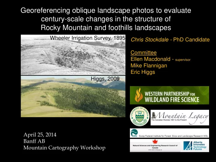
Georeferencing oblique landscape photos to evaluate century-scale changes in the structure of Rocky Mountain and foothills landscapes
Wheeler Irrigation Survey, 1895-1897 Higgs, 2009 Chris Stockdale - PhD Candidate Committee Ellen Macdonald - supervisor Mike Flannigan Eric Higgs April 25, 2014 Banff AB Mountain Cartography Workshop
SLIDE 2
SLIDE 3
History
SLIDE 4 Planning for the future without knowledge of the past is inherently riskier than the alternative.
“We are more likely to use the present to attempt to reconstruct the past, than we are to use the past to understand the present and guide the future.”
SLIDE 5 From: Swetnam et al. 1999. Applied Historical Ecology: Using the past to manage for the future
SLIDE 6 From: Swetnam et al. 1999. Applied Historical Ecology: Using the past to manage for the future
FOREST MANAGEMENT
SLIDE 7 1949
Wheeler 1895 Higgs, 2009
1885 MLP Canada-wide aerial photography 1939 – southern Alberta
SLIDE 8 1949
Wheeler 1895 Higgs, 2009
1885 MLP Canada-wide aerial photography 1939 – southern Alberta
SLIDE 9 1949
Wheeler 1895 Higgs, 2009 Requirements?
- Photographs taken at nadir
- Every pixel = same area*
- Lots of software tools available
SLIDE 10
Rubbersheeting Can’t interpret vegetation after georeferencing
SLIDE 11
Bridgland, 1913
SLIDE 12
SLIDE 13
SLIDE 14
SLIDE 15
From: C. Bozzini, M. Conedera, P. Krebs 2012. A New Monoplotting Tool to Extract Georeferenced Vector Data and Orthorectified Raster Data from Oblique Non-Metric Photographs. International Journal of Heritage in the Digital Era
Digital Monoplotting for Georeferencing Oblique Photography
SLIDE 16
SLIDE 17
SLIDE 18
SLIDE 19
SLIDE 20
SLIDE 21
SLIDE 22
SLIDE 23
SLIDE 24
SLIDE 25
SLIDE 26
SLIDE 27
SLIDE 28
SLIDE 29
SLIDE 30 ACCURACY TEST
- 1. 8 images used
- 2. 21 control points established in each image
- 3. 6 Anchor Points used to georeference the image
- 4. Remaining 15 control points (TEST points) are georeferenced
in Monoplotting tool
- 5. Locations compared to Control Point
SLIDE 31 ACCURACY TEST
- 1. 8 images used
- 2. 21 control points established in each image
- 3. 6 Anchor Points used to georeference the image
- 4. Remaining 15 control points (TEST points) are georeferenced
in Monoplotting tool
- 5. Locations compared to Control Point
SLIDE 32
1.
Polygon based approach
2.
Raster based approach
3.
Hybrid polygon/raster
SLIDE 33
Classify vegetation in plots in Monoplotting Tool
NOTE: Oblique view, MLP image
SLIDE 34
Export spatially referenced objects to ArcGIS (or other GIS)
NOTE: Orthogonal view in GIS
SLIDE 35 NOTE: Orthogonal view in GIS overlain on Orthophoto
SLIDE 36
MLP image
SLIDE 37
Ortho image of same region
SLIDE 38 Viewshed Analysis of image showing what part
- f landscape is visible in
photograph
SLIDE 39
30m grid
Insert spatially referenced grid in Visible landscape
SLIDE 40 30 m 30 m 30 m 30 m 30 m 30 m 30 m 30 m 30 30 m 30 m 30 m 30 m
Export spatially referenced grid to Monoplotting tool for classification of 2009 image
SLIDE 41
1899 image with grid
SLIDE 42
1899
SLIDE 43
1899 2009
SLIDE 44 Initial Final
Grass Shrub Decid. Mixed Conif er Grass
Shrub
1
Deciduous
2 1
Mixed
3 2 1
Conifer
4 3 2 1 Table 1: Vegetation Transition Matrix
SLIDE 45 Initial Final
Grass Shrub Decid. Mixed Conif er Grass
Shrub
1
Deciduous
2 1
Mixed
3 2 1
Conifer
4 3 2 1 Table 1: Vegetation Transition Matrix Figure 1: Raster “change” surface
SLIDE 46 250m 250m 250m 250m 250m 250m
Put plots on landscape
SLIDE 47
SLIDE 48
SLIDE 49 1913 2009
Is 1913 more variable than 2009? Patch sizes, edge to interior, # of patches, fractal dimension, contagion, TPSA Has the leading tree species of the forest changed? Where? Is this to more or less advanced successional species? Is the forest more dense (stem density) in 2009 than 1913? Where is this observed? What were the original conditions? Is the age class distribution of the forest older and more homogenous?
Note: Mock classified imagery
SLIDE 50
Primary Funding Sources Additional Funding Sources In-Kind Support
SLIDE 51
- Bridgland 1912-1913
- Wheeler 1895-1899
- Total 1462 Image
pairs
SLIDE 52 5 km viewshed from all photos
Choose area with extensive view coverage
SLIDE 53
Beaver Mines West Castle Castle Waterton Lakes NP