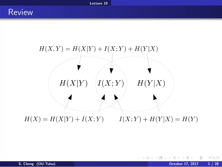
review
play

Review S. Cheng (OU-Tulsa) October 17, 2017 1 / 28 Lecture 10 - PowerPoint PPT Presentation

Lecture 10 Review S. Cheng (OU-Tulsa) October 17, 2017 1 / 28 Lecture 10 Review Conditioning reduces entropy S. Cheng (OU-Tulsa) October 17, 2017 2 / 28 Lecture 10 Review Conditioning reduces entropy Chain rules: H ( X , Y , Z ) S.


  1. Lecture 10 Review S. Cheng (OU-Tulsa) October 17, 2017 1 / 28

  2. Lecture 10 Review Conditioning reduces entropy S. Cheng (OU-Tulsa) October 17, 2017 2 / 28

  3. Lecture 10 Review Conditioning reduces entropy Chain rules: H ( X , Y , Z ) S. Cheng (OU-Tulsa) October 17, 2017 2 / 28

  4. Lecture 10 Review Conditioning reduces entropy Chain rules: H ( X , Y , Z ) = H ( Z ) + H ( Y | X ) + H ( Z | X , Y ) H ( X , Y , U | V ) S. Cheng (OU-Tulsa) October 17, 2017 2 / 28

  5. Lecture 10 Review Conditioning reduces entropy Chain rules: H ( X , Y , Z ) = H ( Z ) + H ( Y | X ) + H ( Z | X , Y ) H ( X , Y , U | V )= H ( X | V ) + H ( Y | X , V ) + H ( U | Y , X , V ) I ( X , Y , Z ; U ) S. Cheng (OU-Tulsa) October 17, 2017 2 / 28

  6. Lecture 10 Review Conditioning reduces entropy Chain rules: H ( X , Y , Z ) = H ( Z ) + H ( Y | X ) + H ( Z | X , Y ) H ( X , Y , U | V )= H ( X | V ) + H ( Y | X , V ) + H ( U | Y , X , V ) I ( X , Y , Z ; U )= I ( X ; U ) + I ( Y ; U | X ) + I ( Z ; U | X , Y ) I ( X , Y , Z ; U | V ) S. Cheng (OU-Tulsa) October 17, 2017 2 / 28

  7. Lecture 10 Review Conditioning reduces entropy Chain rules: H ( X , Y , Z ) = H ( Z ) + H ( Y | X ) + H ( Z | X , Y ) H ( X , Y , U | V )= H ( X | V ) + H ( Y | X , V ) + H ( U | Y , X , V ) I ( X , Y , Z ; U )= I ( X ; U ) + I ( Y ; U | X ) + I ( Z ; U | X , Y ) I ( X , Y , Z ; U | V )= I ( X ; U | V ) + I ( Y ; U | V , X ) + I ( Z ; U | V , X , Y ) Data processing inequality: if X ⊥ Y | Z , S. Cheng (OU-Tulsa) October 17, 2017 2 / 28

  8. Lecture 10 Review Conditioning reduces entropy Chain rules: H ( X , Y , Z ) = H ( Z ) + H ( Y | X ) + H ( Z | X , Y ) H ( X , Y , U | V )= H ( X | V ) + H ( Y | X , V ) + H ( U | Y , X , V ) I ( X , Y , Z ; U )= I ( X ; U ) + I ( Y ; U | X ) + I ( Z ; U | X , Y ) I ( X , Y , Z ; U | V )= I ( X ; U | V ) + I ( Y ; U | V , X ) + I ( Z ; U | V , X , Y ) Data processing inequality: if X ⊥ Y | Z , I ( X ; Y ) ≥ I ( X ; Z ) Independence and mutual information: X ⊥ Y ⇔ S. Cheng (OU-Tulsa) October 17, 2017 2 / 28

  9. Lecture 10 Review Conditioning reduces entropy Chain rules: H ( X , Y , Z ) = H ( Z ) + H ( Y | X ) + H ( Z | X , Y ) H ( X , Y , U | V )= H ( X | V ) + H ( Y | X , V ) + H ( U | Y , X , V ) I ( X , Y , Z ; U )= I ( X ; U ) + I ( Y ; U | X ) + I ( Z ; U | X , Y ) I ( X , Y , Z ; U | V )= I ( X ; U | V ) + I ( Y ; U | V , X ) + I ( Z ; U | V , X , Y ) Data processing inequality: if X ⊥ Y | Z , I ( X ; Y ) ≥ I ( X ; Z ) Independence and mutual information: X ⊥ Y ⇔ I ( X ; Y ) = 0 X ⊥ Y | Z ⇔ S. Cheng (OU-Tulsa) October 17, 2017 2 / 28

  10. Lecture 10 Review Conditioning reduces entropy Chain rules: H ( X , Y , Z ) = H ( Z ) + H ( Y | X ) + H ( Z | X , Y ) H ( X , Y , U | V )= H ( X | V ) + H ( Y | X , V ) + H ( U | Y , X , V ) I ( X , Y , Z ; U )= I ( X ; U ) + I ( Y ; U | X ) + I ( Z ; U | X , Y ) I ( X , Y , Z ; U | V )= I ( X ; U | V ) + I ( Y ; U | V , X ) + I ( Z ; U | V , X , Y ) Data processing inequality: if X ⊥ Y | Z , I ( X ; Y ) ≥ I ( X ; Z ) Independence and mutual information: X ⊥ Y ⇔ I ( X ; Y ) = 0 X ⊥ Y | Z ⇔ I ( X ; Y | Z ) = 0 KL-divergence: KL ( p || q ) � S. Cheng (OU-Tulsa) October 17, 2017 2 / 28

  11. Lecture 10 Review Conditioning reduces entropy Chain rules: H ( X , Y , Z ) = H ( Z ) + H ( Y | X ) + H ( Z | X , Y ) H ( X , Y , U | V )= H ( X | V ) + H ( Y | X , V ) + H ( U | Y , X , V ) I ( X , Y , Z ; U )= I ( X ; U ) + I ( Y ; U | X ) + I ( Z ; U | X , Y ) I ( X , Y , Z ; U | V )= I ( X ; U | V ) + I ( Y ; U | V , X ) + I ( Z ; U | V , X , Y ) Data processing inequality: if X ⊥ Y | Z , I ( X ; Y ) ≥ I ( X ; Z ) Independence and mutual information: X ⊥ Y ⇔ I ( X ; Y ) = 0 X ⊥ Y | Z ⇔ I ( X ; Y | Z ) = 0 x p ( x ) log p ( x ) KL-divergence: KL ( p || q ) � � q ( x ) S. Cheng (OU-Tulsa) October 17, 2017 2 / 28

  12. Lecture 10 Overview This time Identification/Decision trees Random forests Law of Large Number Asymptotic equipartition (AEP) and typical sequences S. Cheng (OU-Tulsa) October 17, 2017 3 / 28

  13. Lecture 10 Identification/Decision tree Vampire database (https://www.youtube.com/watch?v=SXBG3RGr Rc) S. Cheng (OU-Tulsa) October 17, 2017 4 / 28

  14. Lecture 10 Identification/Decision tree Identifying vampire Goal: Design a set of tests to identify vampires Potential difficulties Non-numerical data Some information may not matter Some may matter only sometimes Tests may be costly ⇒ conduct as few as possible S. Cheng (OU-Tulsa) October 17, 2017 5 / 28

  15. Lecture 10 Identification/Decision tree Test trees Complexion Shadow Garlic ? N A R N Y Y P ++ +++ ++ -- --- + --- -- -- -- - + Accent N O H -- - -+ + ++ + : Vampire − : Not vampire S. Cheng (OU-Tulsa) October 17, 2017 6 / 28

  16. Lecture 10 Identification/Decision tree Test trees Complexion Shadow Garlic ? N A R N Y Y P ++ +++ ++ -- --- + --- -- -- -- - + Accent N O H -- - -+ + ++ + : Vampire − : Not vampire How to pick a good test? S. Cheng (OU-Tulsa) October 17, 2017 6 / 28

  17. Lecture 10 Identification/Decision tree Test trees Complexion Shadow Garlic ? N A R N Y Y P ++ +++ ++ -- --- + --- -- -- -- - + Accent N O H -- - -+ + ++ + : Vampire − : Not vampire How to pick a good test? Pick test that identifies most vampires (and non-vampires)! S. Cheng (OU-Tulsa) October 17, 2017 6 / 28

  18. Lecture 10 Identification/Decision tree Sizes of homogeneous sets Complexion Shadow Garlic ? A R N N Y Y P ++ +++ ++ -- --- + --- -- -- -- - + Accent N O H -- - -+ + ++ + : Vampire − : Not vampire S. Cheng (OU-Tulsa) October 17, 2017 7 / 28

  19. Lecture 10 Identification/Decision tree Sizes of homogeneous sets Complexion Shadow Garlic ? A R N N Y Y P ++ +++ ++ -- --- + --- -- -- -- - + Accent N O H -- - -+ + ++ + : Vampire − : Not vampire Shadow: 4 Garlic: 3 Complexion: 2 Accent: 0 S. Cheng (OU-Tulsa) October 17, 2017 7 / 28

  20. Lecture 10 Identification/Decision tree Picking second test Let say we pick “shadow” as the first test after all. Then, for the remaining unclassified individuals, Complexion Garlic Accent N O A R Y N H P -- ++ + - +- +- +- -+ Garlic: 4 Complexion: 2 Accent: 0 S. Cheng (OU-Tulsa) October 17, 2017 8 / 28

  21. Lecture 10 Identification/Decision tree Combined tests Shadow N ? Y Not Garlic Vampire vampire Y N Not Vampire vampire S. Cheng (OU-Tulsa) October 17, 2017 9 / 28

  22. Lecture 10 Identification/Decision tree Combined tests Shadow N ? Y Not Garlic Vampire vampire Y N Not Vampire vampire Problem When our database size increases, none of the test likely to completely separate vampire from non-vampire. All tests will score 0 then. S. Cheng (OU-Tulsa) October 17, 2017 9 / 28

  23. Lecture 10 Identification/Decision tree Combined tests Shadow N ? Y Not Garlic Vampire vampire Y N Not Vampire vampire Problem When our database size increases, none of the test likely to completely separate vampire from non-vampire. All tests will score 0 then. Entropy comes to the rescue! S. Cheng (OU-Tulsa) October 17, 2017 9 / 28

  24. Lecture 10 Identification/Decision tree Conditional entropy as a measure of test efficiency Consider the database is randomly sampled from a distribution. A set is Very homogeneous ≈ high certainty Not so homogenous ≈ high randomness These can be measured with its entropy 0.7 0.6 Shadow 0.5 ? 0.4 N Entropy Y 0.3 0.2 ++-- --- + 0.1 H ( V | S =?) = 1 H ( V | S = Y ) = 0 H ( V | S = N ) = 0 0 0 0.2 0.4 0.6 0.8 1 Pr(Head) S. Cheng (OU-Tulsa) October 17, 2017 10 / 28

  25. Lecture 10 Identification/Decision tree Conditional entropy as a measure of test efficiency Consider the database is randomly sampled from a distribution. A set is Very homogeneous ≈ high certainty Not so homogenous ≈ high randomness These can be measured with its entropy 0.7 0.6 Shadow 0.5 ? 0.4 N Entropy Y 0.3 0.2 ++-- --- + 0.1 H ( V | S =?) = 1 H ( V | S = Y ) = 0 H ( V | S = N ) = 0 0 0 0.2 0.4 0.6 0.8 1 Pr(Head) Remaining uncertainty given the test: 4 8 H ( V | S =?) S. Cheng (OU-Tulsa) October 17, 2017 10 / 28

  26. Lecture 10 Identification/Decision tree Conditional entropy as a measure of test efficiency Consider the database is randomly sampled from a distribution. A set is Very homogeneous ≈ high certainty Not so homogenous ≈ high randomness These can be measured with its entropy 0.7 0.6 Shadow 0.5 ? 0.4 N Entropy Y 0.3 0.2 ++-- --- + 0.1 H ( V | S =?) = 1 H ( V | S = Y ) = 0 H ( V | S = N ) = 0 0 0 0.2 0.4 0.6 0.8 1 Pr(Head) Remaining uncertainty given the test: 8 H ( V | S =?) + 3 4 8 H ( V | S = Y ) S. Cheng (OU-Tulsa) October 17, 2017 10 / 28

  27. Lecture 10 Identification/Decision tree Conditional entropy as a measure of test efficiency Consider the database is randomly sampled from a distribution. A set is Very homogeneous ≈ high certainty Not so homogenous ≈ high randomness These can be measured with its entropy 0.7 0.6 Shadow 0.5 ? 0.4 N Entropy Y 0.3 0.2 ++-- --- + 0.1 H ( V | S =?) = 1 H ( V | S = Y ) = 0 H ( V | S = N ) = 0 0 0 0.2 0.4 0.6 0.8 1 Pr(Head) Remaining uncertainty given the test: 8 H ( V | S =?) + 3 4 8 H ( V | S = Y ) + 1 8 H ( V | S = N ) = 0 . 5 S. Cheng (OU-Tulsa) October 17, 2017 10 / 28

Download Presentation
Download Policy: The content available on the website is offered to you 'AS IS' for your personal information and use only. It cannot be commercialized, licensed, or distributed on other websites without prior consent from the author. To download a presentation, simply click this link. If you encounter any difficulties during the download process, it's possible that the publisher has removed the file from their server.

Recommend


More recommend