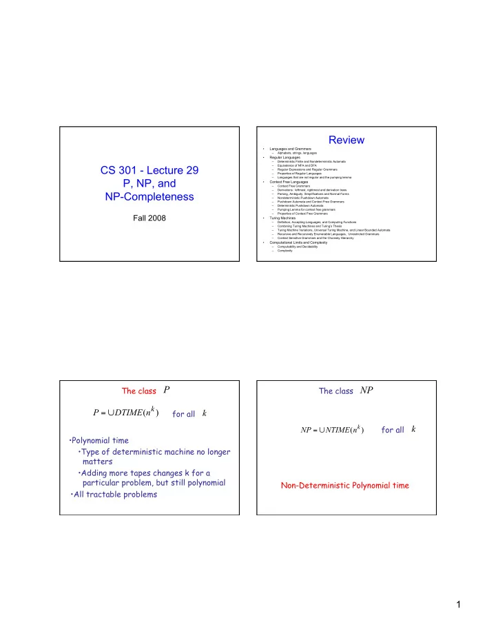
Review Languages and Grammars Alphabets, strings, languages - PDF document

Review • Languages and Grammars – Alphabets, strings, languages • Regular Languages – Deterministic Finite and Nondeterministic Automata CS 301 - Lecture 29 – Equivalence of NFA and DFA – Regular Expressions and Regular Grammars – Properties of Regular Languages – Languages that are not regular and the pumping lemma P, NP, and • Context Free Languages – Context Free Grammars – Derivations: leftmost, rightmost and derivation trees NP-Completeness – Parsing, Ambiguity, Simplifications and Normal Forms – Nondeterministic Pushdown Automata – Pushdown Automata and Context Free Grammars – Deterministic Pushdown Automata – Pumping Lemma for context free grammars – Properties of Context Free Grammars Fall 2008 • Turing Machines – Definition, Accepting Languages, and Computing Functions – Combining Turing Machines and Turing’s Thesis – Turing Machine Variations, Universal Turing Machine, and Linear Bounded Automata – Recursive and Recursively Enumerable Languages, Unrestricted Grammars – Context Sensitive Grammars and the Chomsky Hierarchy • Computational Limits and Complexity – Computability and Decidability – Complexity The class P The class NP ( k P DTIME n ) for all k = ∪ ( k for all k NP NTIME n ) = ∪ • Polynomial time • Type of deterministic machine no longer matters • Adding more tapes changes k for a particular problem, but still polynomial Non-Deterministic Polynomial time • All tractable problems 1

Observation: P = NP ? Open Problem: P ⊆ NP Deterministic WE DO NOT KNOW THE ANSWER Non-Deterministic Polynomial Polynomial Our Three Classic Problems: Why Does P = NP Matter? From Garey and Johnson • Satisfiability “Computers and Intractability” • Hamiltonian Path Function 10 20 30 40 50 60 N 0.0001 s 0.0002 s 0.0003 s 0.0004 s 0.0005 s 0.0006 s • Clique N^2 0.0001 s 0.0004 s 0.0009 s 0.0016 s 0.0025 s 0.0036 s All can be solved in polynomial time using N^5 0.1 s 3.2 s 24.3 s 1.7 min 5.2 min 13.0 min non-deterministic Turing machines. 2^N 0.001 s 1 s 17.9 min 12.7 35.7 366 days years centuries 3^N 0.059 s 58 min 6.5 years 3855 2 X 10^8 10^13 Could they be solved in polynomial time using centuries centuries centuries Common Run Times for Representative Algorithms deterministic Turing machines? 2

Polynomial Time Reductions Polynomial Computable function : f Language A is polynomial time reducible to language B if there is a polynomial For any computes w f ( w ) f computable function such that: in polynomial time w A f ( w ) B ∈ ⇔ ∈ Theorem: Theorem: 3SAT is polynomial time A B reducible to CLIQUE Suppose that is polynomial reducible to . B ∈ P A ∈ P If then . Proof: Let be the machine to accept B M Proof: give a polynomial time reduction A Machine to accept in polynomial time: of one problem to the other w On input : 1. Compute f ( w ) M 2. Run on input f ( w ) 3

3CNF formula: Clique: A 5-clique ( x x x ) ( x x x ) ( x x x ) ( x x x ) ∨ ∨ ∧ ∨ ∨ ∧ ∨ ∨ ∧ ∨ ∨ 1 2 3 3 5 6 3 6 4 4 5 6 Each clause has three literals Language: CLIQUE = { : Given a graph G , k < > does G contains a -clique} k G w w 3SAT ={ : is a satisfiable 3CNF formula} Again, no obvious deterministic polynomial time algorithm….. ( x x x ) ( x x x ) ( x x x ) ∨ ∨ ∧ ∨ ∨ ∧ ∨ ∨ 1 1 2 1 2 2 1 2 3 ( x x x ) ( x x x ) ( x x x ) ∨ ∨ ∧ ∨ ∨ ∧ ∨ ∨ x 1 = 1 1 2 1 2 2 1 2 3 1 x 0 = 2 x 1 = x 3 x x x x x 2 2 1 2 1 2 x x x x 1 1 1 1 x x x x 1 2 1 2 x x x x 2 3 2 3 4

Theorem: Vertex Cover is polynomial time Clique: reducible to CLIQUE A 5-clique Proof: give a polynomial time reduction CLIQUE = { : Given a graph G , k < > of one problem to the other does G contains a -clique} k G Again, no obvious deterministic polynomial time algorithm….. Reduction: Cliques and Covers: Given a Graph G, define its complement Gc Let V1 = the Clique found in Gc. Claim (V – V1) is a cover in G. All vertices in G are vertices in Gc. Pick an arbitrary edge (u,v) in G. An edge (u,v) is in Gc if and only if (u,v) is not an edge in G. Suppose neither u or v is in (V-V1). ⇒ Both u and v are V1 1) Convert G into Gc… an easy step. ⇒ Both u and v are in a clique in Gc ⇒ there must be an edge (u,v) in Gc 2) Ask whether Gc has a clique of size K? ⇒ there must not be an edge (u,v) in G But (u,v) was an edge in G! 5

Theorem: (ANY PROBLEM IN NP) is polynomial time NP-Completeness reducible to CLIQUE A problem is NP-complete if: • It is in NP Clique is an NP-complete problem. • Every NP problem is reduced to it Solve Clique in polynomial time and you (in polynomial time) solve all NP problems in polynomial time. Observation: Observation: If we can solve any NP-complete problem If we prove that in Deterministic Polynomial Time (P time) we cannot solve an NP-complete problem then we know: in Deterministic Polynomial Time (P time) then we know: P = NP P ≠ NP 6

Observations: Cook’s Theorem: It is unlikely(??) that NP-complete The satisfiability problem is NP-complete problems are in P The NP-complete problems have Sketch of Proof: exponential time algorithms Convert a Non-Deterministic Turing Machine to a Boolean expression Approximations of these problems in conjunctive normal form are in P Other NP-Complete Problems: Vertex Cover = { : Given a graph G , k G < > does G contains a size cover? } k • The Traveling Salesperson Problem A cover is a set of vertices in G such that • Vertex cover for every edge (u,v) in G, at least one of u and v belongs to G. • Hamiltonian Path All the above are reduced to the satisfiability problem 7

Where to Go From Here? Where to Go From Here? NP Hard: drop requirement problem is in NP, but still The View We Have From CS 301 “as hard as” an NP-complete problem. RP: Randomized Computations PSPACE: Polynomial Space NP Incorporating distributed computations. See Papadimitriou, “Computational Complexity” P We have established a starting point for a very rich analysis of complexity in both time and space. Where to Go From Here? What’s Next A larger view of complexity theory • Read – Linz Chapter 1,2.1, 2.2, 2.3, (skip 2.4), 3, 4, 5, 6.1, 6.2, (skip 6.3), 7.1, 7.2, 7.3, (skip 7.4), 8, 9, 10, 11, 12.1, 12.2, (skip 12.3, 12.4, 12.5, 13), 14.1, 14.2, and 14.3 – JFLAP Chapter 1, 2.1, (skip 2.2), 3, 4, 5, 6, 7, (skip 8), 9, (skip 10), 11 • Next Lecture Topics – Review for Final Exam • Final exam Friday 12/19 – Closed book, but you may bring one sheet of 8.5 x 11 inch paper with any notes you like. • Homework – Homework 15 (repeat of previous homework problems) Due Today – Homework 16 = study for the final!! 8