Review of Model Existence Theorem MAT309, Fall 2019 Completeness - - PowerPoint PPT Presentation

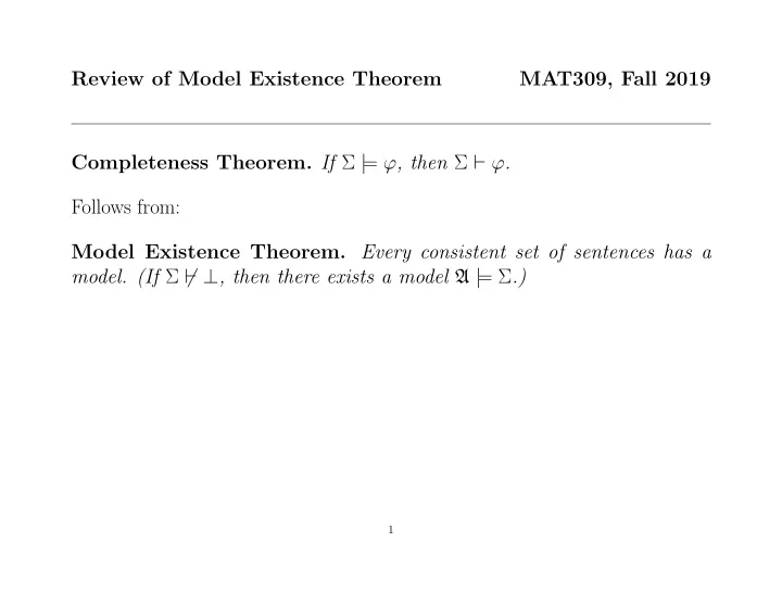
Review of Model Existence Theorem MAT309, Fall 2019 Completeness Theorem. If Σ | = ϕ, then Σ ⊢ ϕ. Follows from: Model Existence Theorem. Every consistent set of sentences has a

• model. (If Σ ⊢ ⊥, then there exists a model A |

= Σ.)

1

Completeness Theorem. If Σ | = ϕ, then Σ ⊢ ϕ. Model Existence Theorem. If Σ ⊢ ⊥, then ∃ a model A | = Σ. Proof of Completeness Thm from Model Existence Thm.

• 1. Suffices to prove Completeness Theorem in the case where Σ is a set of

sentences and ϕ is a sentence. (Follows from the fact that {α} ⊢ ∀α and {∀xα} ⊢ α for all formulas α.)

• 2. Assume Σ |

= ϕ. Then A | = Σ ⇒ A | = ϕ for all structures A. Therefore, Σ ∪ {¬ϕ} has no models. By Model Existence Theorem, Σ ∪ {¬ϕ} ⊢ ⊥. By Deduction Theorem, Σ ⊢ (¬ϕ → ⊥). By (PC) rule, Σ ⊢ ϕ (via the tautology (¬P → False) → P)). Q.E.D.

2

Proof of the Model Existence Theorem

3

Let L be a countable language. (The case of uncountable languages uses Zorn’s Lemma, as explained in tutorial.) Let Σ be a consistent set of L-sentences. We will construct a model A | = Σ.

4

Let L be a countable language. (The case of uncountable languages uses Zorn’s Lemma, as explained in tutorial.) Let Σ be a consistent set of L-sentences. We will construct a model A | = Σ. We first construct a language L′ = L∪{countably many new constant symbols} and a set of L′-sentences Σ such that (1) Σ ⊆ Σ, (2)

• Σ is consistent,

(3)

• Σ contains a Henkin axiom (∃xθ) → θx

c for each L′-sentence ∃xθ.

5

Let L be a countable language. (The case of uncountable languages uses Zorn’s Lemma, as explained in tutorial.) Let Σ be a consistent set of L-sentences. We will construct a model A | = Σ. We first construct a language L′ = L∪{countably many new constant symbols} and a set of L′-sentences Σ such that (1) Σ ⊆ Σ, (2)

• Σ is consistent,

(3)

• Σ contains a Henkin axiom (∃xθ) → θx

c for each L′-sentence ∃xθ.

We then complete Σ to a maximal consistent set of L′-sentences Σ′ (by adding either ϕ or ¬ϕ one-at-a-time for each L′-sentence ϕ). In addition to properties (1)–(3), Σ′ has the property: (4) For every L′-sentence ϕ, ϕ ∈ Σ′ ⇐ ⇒ Σ′ ⊢ ϕ ⇐ ⇒ ¬ϕ / ∈ Σ′ ⇐ ⇒ Σ′ ⊢ ¬ϕ.

6

The L′-Structure A: We define an equivalence relation ∼ on {variable-free L′-terms} by t ∼ u

def

⇐ ⇒ (t = u) ∈ Σ′ ⇐ ⇒ Σ′ ⊢ (t = u).

7

The L′-Structure A: We define an equivalence relation ∼ on {variable-free L′-terms} by t ∼ u

def

⇐ ⇒ (t = u) ∈ Σ′ ⇐ ⇒ Σ′ ⊢ (t = u). CLAIM: ∼ is an equivalence relation. PROOF: Here is the argument that ∼ is symmetric: Assume t ∼ u. Then Σ′ ⊢ (t = u). We know ⊢ (∀x)(∀y)[(x = y) → (y = x)] (from Chapter 2). Therefore, ⊢ (t = u) → (u = t) by (Q1) axiom and (PC) rule. Therefore, Σ′ ⊢ (u = t) by (PC) rule; hence u ∼ t.

8

The L′-Structure A: We define an equivalence relation ∼ on {variable-free L′-terms} by t ∼ u

def

⇐ ⇒ (t = u) ∈ Σ′ ⇐ ⇒ Σ′ ⊢ (t = u). Let A be the following structure:

• A := {[t]∼ : t is a variable-free L′-term}

(universe of A)

• cA := [c]∼

for each constant symbol c

• f A([t1]∼, . . . , [tn]∼) := [ft1 . . . tn]∼

for each n-ary f

• ([t1]∼, . . . , [tn]∼) ∈ RA

def

⇐ ⇒ Rt1 . . . tn ∈ Σ′ for each n-ary R

9

The L′-Structure A: We define an equivalence relation ∼ on {variable-free L′-terms} by t ∼ u

def

⇐ ⇒ (t = u) ∈ Σ′ ⇐ ⇒ Σ′ ⊢ (t = u). Let A be the following structure:

• A := {[t]∼ : t is a variable-free L′-term}

(universe of A)

• cA := [c]∼

for each constant symbol c

• f A([t1]∼, . . . , [tn]∼) := [ft1 . . . tn]∼

for each n-ary f

• ([t1]∼, . . . , [tn]∼) ∈ RA

def

⇐ ⇒ Rt1 . . . tn ∈ Σ′ for each n-ary R NOTE: To show that f A and RA are well-defined, we must show that if ti ∼ ui for i = 1, . . . , n, then

• [ft1 . . . tn]∼ = [fu1 . . . un]∼ (that is, (ft1 . . . tn = fu1 . . . un) ∈ Σ′) and
• Rt1 . . . tn ∈ Σ′ ⇐

⇒ Ru1 . . . un ∈ Σ′.

10

Proposition 3.2.6. For every L′-sentence ϕ, we have ϕ ∈ Σ′ ⇐ ⇒ A | = ϕ.

11

Proposition 3.2.6. For every L′-sentence ϕ, we have ϕ ∈ Σ′ ⇐ ⇒ A | = ϕ. The Model Existence Theorem follows from Prop 3.2.5 as follows:

• As a consequence of Prop 3.2.6, A |

= Σ′.

• Since Σ ⊂

Σ ⊂ Σ′, it follows that A | = Σ.

• If we ignore that interpretation of constant symbols in L′ \ L, then the

“reduct” A|L is a model of Σ in the original language L.

12

Proposition 3.2.6. For every L′-sentence ϕ, we have ϕ ∈ Σ′ ⇐ ⇒ A | = ϕ.

• PROOF. We argue by induction on the complexity of ϕ.

As usual, we consider five cases:

• 1. ϕ :≡ Rt1 . . . tn

(base case)

• 2. ϕ :≡ t1 = t2

(base case)

• 3. ϕ :≡ ¬α

(easy induction step)

• 4. ϕ :≡ α ∨ β

(easy induction step)

• 5. ϕ :≡ ∀xα

(non-trivial induction step)

13

Proposition 3.2.6. For every L′-sentence ϕ, we have ϕ ∈ Σ′ ⇐ ⇒ A | = ϕ. CASE 1. ϕ :≡ Rt1 . . . tn We have ϕ ∈ Σ′ ⇐ ⇒ ([t1]∼, . . . , [tn]∼) ∈ RA ⇐ ⇒ A | = ϕ.

14

Proposition 3.2.6. For every L′-sentence ϕ, we have ϕ ∈ Σ′ ⇐ ⇒ A | = ϕ. CASE 2. ϕ :≡ t1 = t2 We use the fact (shown by induction) that s(t) = [t]∼ for every variable-free term t and s : Vars → A. It follows: A | = ϕ ⇐ ⇒ A | = ϕ[s] for every s : Vars → A ⇐ ⇒ s(t1) = s(t2) for every s : Vars → A ⇐ ⇒ [t1]∼ = [t2]∼ (since s(t) = [t]∼) ⇐ ⇒ (t1 = t2) ∈ Σ′ ⇐ ⇒ ϕ ∈ Σ′.

15

Proposition 3.2.6. For every L′-sentence ϕ, we have ϕ ∈ Σ′ ⇐ ⇒ A | = ϕ. CASE 3. ϕ :≡ ¬α A | = ϕ ⇐ ⇒ A | = α ⇐ ⇒ α / ∈ Σ′ (induction hypothesis applied to α) ⇐ ⇒ ¬α ∈ Σ′ (since α ∈ Σ′ ⇐ ⇒ ¬α ∈ Σ′) ⇐ ⇒ ϕ ∈ Σ′.

16

Proposition 3.2.6. For every L′-sentence ϕ, we have ϕ ∈ Σ′ ⇐ ⇒ A | = ϕ. CASE 4. ϕ :≡ α ∨ β Another trivial induction step.

17

Proposition 3.2.6. For every L′-sentence ϕ, we have ϕ ∈ Σ′ ⇐ ⇒ A | = ϕ. CASE 5. ϕ :≡ ∀xα ϕ ∈ Σ′ = ⇒ A | = ϕ

18

Proposition 3.2.6. For every L′-sentence ϕ, we have ϕ ∈ Σ′ ⇐ ⇒ A | = ϕ. CASE 5. ϕ :≡ ∀xα ϕ ∈ Σ′ = ⇒ A | = ϕ Assume ϕ ∈ Σ′. To show A | = ϕ, we must show A | = ϕ[s] for every s : Vars → A, that is, A | = α[s[x|a]] for every s : Vars → A and a ∈ A.

19

Proposition 3.2.6. For every L′-sentence ϕ, we have ϕ ∈ Σ′ ⇐ ⇒ A | = ϕ. CASE 5. ϕ :≡ ∀xα ϕ ∈ Σ′ = ⇒ A | = ϕ Assume ϕ ∈ Σ′. To show A | = ϕ, we must show A | = ϕ[s] for every s : Vars → A, that is, A | = α[s[x|a]] for every s : Vars → A and a ∈ A. Fix any s : Vars → A and a = [t]∼ ∈ A. We have A | = α[s[x|a]] ⇐ ⇒ A | = α[s[x|s(t)]] (since s(t) = [t]∼ = a) ⇐ ⇒ A | = αx

t [s]

(by Theorem 2.6.2) ⇐ ⇒ A | = αx

t

(since αx

t is a sentence).

20

Proposition 3.2.6. For every L′-sentence ϕ, we have ϕ ∈ Σ′ ⇐ ⇒ A | = ϕ. CASE 5. ϕ :≡ ∀xα ϕ ∈ Σ′ = ⇒ A | = ϕ Assume ϕ ∈ Σ′. To show A | = ϕ, we must show A | = ϕ[s] for every s : Vars → A, that is, A | = α[s[x|a]] for every s : Vars → A and a ∈ A. Fix any s : Vars → A and a = [t]∼ ∈ A. We have A | = α[s[x|a]] ⇐ ⇒ A | = α[s[x|s(t)]] (since s(t) = [t]∼ = a) ⇐ ⇒ A | = αx

t [s]

(by Theorem 2.6.2) ⇐ ⇒ A | = αx

t

(since αx

t is a sentence).

Since ϕ ∈ Σ′, we have Σ′ ⊢ ∀xα, hence Σ ⊢ αx

t by (Q1) axiom and (PC) rule.

(OBS: Since t is variable-free, it is substitutable for x.)

21

Proposition 3.2.6. For every L′-sentence ϕ, we have ϕ ∈ Σ′ ⇐ ⇒ A | = ϕ. CASE 5. ϕ :≡ ∀xα ϕ ∈ Σ′ = ⇒ A | = ϕ Assume ϕ ∈ Σ′. To show A | = ϕ, we must show A | = ϕ[s] for every s : Vars → A, that is, A | = α[s[x|a]] for every s : Vars → A and a ∈ A. Fix any s : Vars → A and a = [t]∼ ∈ A. We have A | = α[s[x|a]] ⇐ ⇒ A | = α[s[x|s(t)]] (since s(t) = [t]∼ = a) ⇐ ⇒ A | = αx

t [s]

(by Theorem 2.6.2) ⇐ ⇒ A | = αx

t

(since αx

t is a sentence).

Since ϕ ∈ Σ′, we have Σ′ ⊢ ∀xα, hence Σ ⊢ αx

t by (Q1) axiom and (PC) rule.

(OBS: Since t is variable-free, it is substitutable for x.) Therefore, αx

t ∈ Σ′. By induction hypothesis applied to αx t , it follows that

A | = αx

t . Hence, A |

= ϕ.

22

Proposition 3.2.6. For every L′-sentence ϕ, we have ϕ ∈ Σ′ ⇐ ⇒ A | = ϕ. CASE 5. ϕ :≡ ∀xα ϕ / ∈ Σ′ = ⇒ A | = ϕ

23

Proposition 3.2.6. For every L′-sentence ϕ, we have ϕ ∈ Σ′ ⇐ ⇒ A | = ϕ. CASE 5. ϕ :≡ ∀xα ϕ / ∈ Σ′ = ⇒ A | = ϕ Assume ϕ / ∈ Σ′. Then ¬ϕ ∈ Σ′, hence Σ′ ⊢ ¬ϕ :≡ ¬∀xα, hence Σ′ ⊢ ∃x¬α.

24

Proposition 3.2.6. For every L′-sentence ϕ, we have ϕ ∈ Σ′ ⇐ ⇒ A | = ϕ. CASE 5. ϕ :≡ ∀xα ϕ / ∈ Σ′ = ⇒ A | = ϕ Assume ϕ / ∈ Σ′. Then ¬ϕ ∈ Σ′, hence Σ′ ⊢ ¬ϕ :≡ ¬∀xα, hence Σ′ ⊢ ∃x¬α. The set Σ (and hence also Σ′) contains a Henkin axiom (∃x¬α) → (¬α)x

c.

25

Proposition 3.2.6. For every L′-sentence ϕ, we have ϕ ∈ Σ′ ⇐ ⇒ A | = ϕ. CASE 5. ϕ :≡ ∀xα ϕ / ∈ Σ′ = ⇒ A | = ϕ Assume ϕ / ∈ Σ′. Then ¬ϕ ∈ Σ′, hence Σ′ ⊢ ¬ϕ :≡ ¬∀xα, hence Σ′ ⊢ ∃x¬α. The set Σ (and hence also Σ′) contains a Henkin axiom (∃x¬α) → (¬α)x

c.

Hence Σ′ ⊢ (∃x¬α) → (¬α)x

• c. Therefore, by (PC) rule (modus ponens),

Σ′ ⊢ (¬α)x

c.

By the induction hypothesis applied to the sentence (¬α)x

c, we have A |

= (¬α)x

c.

26

Proposition 3.2.6. For every L′-sentence ϕ, we have ϕ ∈ Σ′ ⇐ ⇒ A | = ϕ. CASE 5. ϕ :≡ ∀xα ϕ / ∈ Σ′ = ⇒ A | = ϕ Assume ϕ / ∈ Σ′. Then ¬ϕ ∈ Σ′, hence Σ′ ⊢ ¬ϕ :≡ ¬∀xα, hence Σ′ ⊢ ∃x¬α. The set Σ (and hence also Σ′) contains a Henkin axiom (∃x¬α) → (¬α)x

c.

Hence Σ′ ⊢ (∃x¬α) → (¬α)x

• c. Therefore, by (PC) rule (modus ponens),

Σ′ ⊢ (¬α)x

c.

By the induction hypothesis applied to the sentence (¬α)x

c, we have A |

= (¬α)x

c.

It follows that A | = ∃x¬α, hence A | = ¬∃x¬α, hence A | = ϕ as required. Q.E.D.

27

Model Existence Theorem. Every consistent set of sentences has a model. Completeness Theorem. If Σ | = ϕ, then Σ ⊢ ϕ. Compactness Theorem. Σ | = ϕ iff Σ0 | = ϕ for some finite Σ0 ⊆ Σ.

28

The Compactness Theorem

29

COMPACTNESS THEOREM (Theorem 3.3.1) Let Σ be any set of

• formulas. Then Σ has a model (a.k.a. it is “satisfiable”) if, and only if, every

finite subset of Σ has a model.

30

COMPACTNESS THEOREM (Theorem 3.3.1) Let Σ be any set of

• formulas. Then Σ has a model (a.k.a. it is “satisfiable”) if, and only if, every

finite subset of Σ has a model.

• Proof. (⇒) trivial: If A |

= Σ, then A | = Σ0 for every finite Σ0 ⊆ Σ.

31

COMPACTNESS THEOREM (Theorem 3.3.1) Let Σ be any set of

• formulas. Then Σ has a model (a.k.a. it is “satisfiable”) if, and only if, every

finite subset of Σ has a model.

• Proof. (⇒) trivial: If A |

= Σ, then A | = Σ0 for every finite Σ0 ⊆ Σ. (⇐): Assume that Σ has no model. We will show that some finite Σ0 ⊆ Σ has no model.

32

COMPACTNESS THEOREM (Theorem 3.3.1) Let Σ be any set of

• formulas. Then Σ has a model (a.k.a. it is “satisfiable”) if, and only if, every

finite subset of Σ has a model.

• Proof. (⇒) trivial: If A |

= Σ, then A | = Σ0 for every finite Σ0 ⊆ Σ. (⇐): Assume that Σ has no model. We will show that some finite Σ0 ⊆ Σ has no model. Since Σ has no model, this means Σ | = ⊥. By the Completeness Theorem (or the contrapositive of the Model Existence Theorem), it follows that Σ ⊢ ⊥. That is, there exists a deduction (δ1, . . . , δn) of ⊥ from Σ.

33

COMPACTNESS THEOREM (Theorem 3.3.1) Let Σ be any set of

• formulas. Then Σ has a model (a.k.a. it is “satisfiable”) if, and only if, every

finite subset of Σ has a model.

• Proof. (⇒) trivial: If A |

= Σ, then A | = Σ0 for every finite Σ0 ⊆ Σ. (⇐): Assume that Σ has no model. We will show that some finite Σ0 ⊆ Σ has no model. Since Σ has no model, this means Σ | = ⊥. By the Completeness Theorem (or the contrapositive of the Model Existence Theorem), it follows that Σ ⊢ ⊥. That is, there exists a deduction (δ1, . . . , δn) of ⊥ from Σ. Let Σ0 := Σ ∩ {δ1, . . . , δn}. Observe that Σ0 is a finite set and Σ0 ⊢ ⊥ (since the same sequence (δ1, . . . , δn) is a deduction of ⊥ from Σ0). Therefore, Σ0 | = ⊥ by the Soundness Theorem. This means that Σ0 has no model, as required.

34

COMPACTNESS THEOREM (Theorem 3.3.1) Let Σ be any set of

• formulas. Then Σ has a model (a.k.a. it is “satisfiable”) if, and only if, every

finite subset of Σ has a model. Corollary 3.2.2. Σ | = ϕ iff Σ0 | = ϕ for some finite subset Σ0 of Σ.

35

In lectures and tutorial, we discussed several applications of the Compactness Theorem:

• 1. If Σ has finite models of size ≥ n for every n ∈ N, then Σ has an infinite

model.

• 2. Every set S admits a linear order <.
• 3. K¨
• nig’s Infinity Lemma (Example 3.3.8): Every infinite tree contains a

vertex of infinite degree or an infinite simple path.

• 4. Wang tiles (wikipedia): A set of Wang tiles can tile the plane iff it can tile

any n × n region.

• 5. The 4-Color Theorem for infinite planar graphs (Examples 3.3.6)
• 6. Non-standard models of arithmetic (Example 3.3.3)
• 7. Non-standard analysis (Example 3.3.5)
• 8. We briefly mentioned (a version of) the L¨
• wenheim-Skolem Theorems (§3.4)
• 9. Infinite Ramsey Theorem ⇒ Finite Ramsey Theorem (homework problem)

36