Report from Vortex Induced Vibration Specialist Committee of the - - PowerPoint PPT Presentation

Report from Vortex Induced Vibration Specialist Committee of the 25th ITTC

Contents

• Members & meetings
• Introduction
• Review

– Ocean current – Experimental methods – Numerical prediction models

• Assessments
• Benchmark bench study
• Technical conclusions

Members of the VIV Committee of the 25th ITTC

• Halvor Lie, MARINTEK, Norway (Chairman)
• Elena Ciappy, INSEAN, Italy
• Shan Huang, University of Glasgow & Strathclyde, UK
• Jung-Chun Suh, SNU, Korea
• Xiong-Liang Yao, HEU, China
• Chang-Kyu Rheem, University of Tokyo, Japan
• Don Spencer, Oceanic, Canada

Four committee meetings

• INSEAN, Italy, March 2006
• Harbin Engineering University, China, September 2006
• MARINTEK, Trondheim, Norway, October 2007
• University of Tokyo, Japan, February 2008

Recommendation given to the committee

• 1. Conduct an in-depth review of Vortex Induced

Vibration (VIV) and Vortex Induced Motion (VIM), including experimental and numerical modeling. Identify and report on technology gaps and make recommendations for future work.

• 2. Conduct an assessment of different prediction methods,

and make recommendations on their application and limitations.

• 3. Define and initiate a specific benchmark case study to

be used to compare different experimental techniques. This could be based upon existing or new experiments.

Vortex Induced Vibrations

Strouhal frequency: fs = St U / D Example: Riser with D = 0.3 m, U = 1.5 m/s: fs = 1 Hz, Ts = 1 s Example: SPAR with D = 30 m, U = 1.5 m/s: fs = 0.01 Hz, Ts = 100 s Current

In-line oscillations A≈D/4

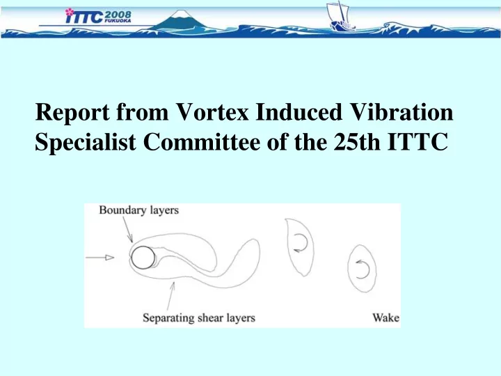
Vortex shedding

Cross-flow oscillations A≈D

Consequences of VIV

• Risk of fatigue damage
• Increased current drag

VIV problem areas

Strouhal Number vs. Reynolds Number

MS & CFD FS

Experimental Methods

• Two different set-ups

– 2D tests with rigid cylinder with various geometrical shapes that are either elastic mounted, free to move or with forced motion and towed in still water – 3D test with long elastic cylinder with varying geometries and boundary conditions, free to

• vibrate. Various flow condition and current

profiles may be arranged

Cross-Flow VIV Behaviour

Lift Coefficient from Forced Motion 2D Test (Gopalkrishnan)

ˆ /

• sc

f f D U = / A D

Riser eigenmodes

To each mode, n, there corresponds an eigen- frequency, fn . The riser will

• scillate when the Strouhal

frequency is close to an eigenfrequency: fn ≈ fs = St⋅U/D Hence, the speed of the current will determine which mode (n) will respond.

5 10 15 20 25 30 35 40 −1 −0.9 −0.8 −0.7 −0.6 −0.5 −0.4 −0.3 −0.2 −0.1

n: 1 2 3 4 5 6 7 ....

.....

f1 f2 f3 f4 f5 f6 f7 ....

Complex hydroelastic interactions for long risers in sheared flow

f1 f2 f3 f4 f5 f6

Strouhal Frequency fs = St U/d Current profile, U Riser

Natural frequencies:

Competing modes

Varying current profile: Many possible frequencies of oscillation exist. ”Competition” between modes. Difficult to predict frequency.

CF and IL fatigue vs. tow speed for bare riser in uniform flow

• Max. fatigue damage vs. tow speed

1.00E-11 1.00E-10 1.00E-09 1.00E-08 1.00E-07 1.00E-06 1.00E-05 1.00E-04 1.00E-03 1.00E-02 1.00E-01 1.00E+00 0.00 0.50 1.00 1.50 2.00 2.50 Velocity [m/s] D [1/yrs] Bare 17.5D0.25D 5D0.14D

Systematic study of triple-start straked risers

• 240
• 230
• 220
• 210
• 200
• 190
• 180
• 170
• 160
• 150
• 140
• 130
• 120
• 110
• 100
• 90
• 80
• 70
• 60
• 50
• 40
• 30
• 20
• 10

• 180
• 160
• 140
• 120
• 100
• 80
• 60
• 40
• 20

• 0.250
• 0.217
• 0.183
• 0.150
• 0.117
• 0.083
• 0.050
• 0.017

3D velocity vector plot based on the PIV measurements Arrows present velocity in the paper plane Colours the velocity normal to paper plane

Soft marine growth (slimy marine grass)

Soft marine growth on a real riser Soft marine as a model

Hard marine growth (Shell, wart barnacle, etc.)

Hard marine growth on a real riser Hard marine growth as modeled

Instability of Faired Riser, 3 D Test

Fairing Riser

Ocean currents and measurement

• High variability of the current presents new

requirements to the way that the ocean currents should be modelled

• Design current profiles are often established based

upon field measurements of the current velocities at a number of current meters arranged along a vertical line at the location

• Reliable methods for obtaining design current

conditions for a given deep water location have yet to be developed

Semi-empirical VIV models

• Semi-empirical models for VIV response

analysis use the hydrodynamic force coefficients such as drag coefficient, lift coefficient, added mass coefficient and hydrodynamic damping coefficient.

• These coefficients are normally obtained

from rigid-cylinder model tests with forced motions

Semi-empirical VIV models - Commercial software

Shear7 (MIT) VIVA (MIT) VIVANA (MARINTEK)

Cross-flow oscillations only Adequate prediction of response for circular cross sections for low modal cases when exposed to 2D uniform and mildly sheared currents Large uncertainties in fatigue, need high SF Further improvements needed for other cases with non- circular cross sections, higher modal responses (>10th mode) and more complex current profiles

Wake Oscillator Models

• Use a van der Pol oscillator to represent the

time-varying force, which is coupled to body motion

• The models generally have the following

characteristics

– Oscillator is self-exciting and self-limiting – Natural frequency of the oscillator is proportional to the free stream velocity such that the Strouhal relationship is satisfied – Cylinder motion interacts with the oscillator

Computational Fluid Dynamics

• Stationary cylinder

– Direct Navier Stokes (DNS) for Rn<10000 – Large Eddy Simulations (LES) – Reynolds-Averaged Navier-Stokes (RANS)

Computational Fluid Dynamics

• Oscillating cylinder

– A certain number of 2D numerical simulations

• n VIV can be found

– 3D simulations are quite limited and usually refer to low Reynolds number values and small aspect ratio. – Direct Navier Stokes (DNS) – Large Eddy Simulations (LES) – Reynolds-Averaged Navier-Stokes (RANS) – Discrete Vortex Method (DVM)

Validation of prediction models

Key results from blind test, Chaplin et al. (2005)

Empirical codes Empirical codes

CFD

Validation of prediction models

• Summary of comparison between laboratory measurements

and blind predictions of 11 numerical models, ref. Chaplin et al. (2005)

– In general, empirical models were more successful in predicting CF displacements and curvatures than CFD codes – Big spread of the results regarding CF curvature predictions and almost all are not conservative – IL displacement is underestimated by all numerical models – IL curvature calculated only by CFD codes but it is in very poor agreement with the measurements.

Define and initiate a specific benchmark case study

A remaining task, but

• OMAE has ongoing activity for benchmarking VIV, where

numerical prediction results will be compared with experimental results

• Suggest that ITTC should establish cooperation with

OMAE on the benchmark activity, where ITTC can provide valuable experimental data to OMAE

• Define and initiate a benchmark model test study, where

results from various experiments will be compared. The recommended test set-up compromises a rigid cylinder which is elastically mounted and free to move.

Define and initiate a specific benchmark case study

Example of possible test set-up though different test set-ups are permissible

Technical Conclusions

– General trends

• Oil and gas industry strong focus on VIV because VIV can be a

detrimental factor in offshore field developments with potential huge economic losses and reduced safety, particularly in deep

• water. Marine risers, free spanning pipelines, tethers and floating

vessels are typical structures subjected to VIV

• VIV difficult subject with a complex structural-hydrodynamic
• interaction. Generally less well understood than other marine

loading processes. Considered to be correspondingly less accurate

• During the last decade there has been a great deal of VIV focused

research activities, both in the industry and in the academia

Technical Conclusions

– Experimental studies

• Important for determination of coefficients used in semi-empirical

codes

• Important for verification of numerical methods/studies
• Relatively large uncertainties of various parameters (i.e. Rn, 3D

current, IL effect). Their influences on VIV are not well understood

• Most of experiments are done in the sub-critical Rn regime
• Lack of data for higher, full-scale Rn regime
• Demand for full-scale measured data with coherent high quality

environmental and response data

• The experimental results depend on the test set-up, but no

recommendations/guidelines exist

Technical Conclusions

– Prediction methods

• CFD still considered as research tool with prohibitive demand for

CPU and large uncertainties. However, probably the method yet to realize its potential in the future

• Semi-empirical prediction methods are currently used in the

design of marine risers and other slender structures. In the last decade the methods have been improved

– Prediction of response for low modal cases when exposed to 2D uniform and mildly sheared currents appear to be adequate – For other cases the methods need further improvements – Only the CF VIV response is normally dealt with. Recommended to incorporate IL response in future models

Suggestion to further activities

The ITTC VIV committee suggest to continue its activity for one more term with the following tasks:

• 1. Define and initiate a benchmark model test study, where results

from various experiments will be compared. The recommended test set-up compromises a rigid cylinder which is elastically mounted and free to move.

• 2. Recommended that ITTC should establish cooperation with

OMAE on the benchmark activity, where ITTC can provide valuable experimental data to OMAE

Suggestion to further activities

• 2. Evaluate need for guidelines on VIV experiment
• 3. Evaluate need for defining and standardizing VIV related

nomenclatures

• 4. Update VIV review including assessment of experimental and

numerical prediction models and the proposed benchmark study activities of ITTC VIV Committee and OMAE

Thank You