Regularization of Error Covariances Nancy Nichols * Joanne Waller*, - - PowerPoint PPT Presentation

Nancy Nichols*

Joanne Waller*, Jemima Tabeart*, Sarah Dance*, Amos Lawless*

*

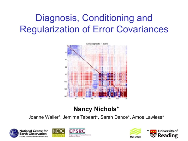
Diagnosis, Conditioning and Regularization of Error Covariances

Minimize with respect to initial state :

Optimal Bayesian Estimate

The solution at the minimum, xa , is the analysis.

Outline

• Observation Errors
• Diagnosing Observation Error Covariances
• Incorporating Observation Errors in DA
• Sensitivity of the Analysis
• Regularization
• Conclusions

• 1. Observation Errors
• 1. Observation Errors

Observation Error Covariance Matrix

• Observation errors have been

assumed to be uncorrelated in data assimilation.

• Observation errors in real data

are found to be correlated.

(Stewart et al, 2009, 2013; Bormann et al, 2010; Waller et al, 2013, 2014a.)

• Using observation error

correlations in data assimilation is shown to improve the state estimate.

(Stewart et al, 2008, 2010, 2014; Weston, 2014.)

Observation Errors

Observation Errors

Four main sources of observation errors, which are time and spatially varying:

Waller et al, 2014a; Stewart, 2014; Hodyss & Nichols, 2014

It is important to be able to account for observation error correlations:

• Avoids thinning (high resolution forecasting)
• More information content
• Better analysis accuracy
• Improved forecast skill scores

Observation Errors

Stewart et al, 2008, 2009, 2010, 2013, 2014; Bormann et al, 2010; Waller et al, 2013, 2014a; Weston, 2014

• 1. Observation Errors
• 2. Diagnosing Observation

Error Covariances

DBCP Diagnostic (Desroziers et al, 2005)

Let

DBCP Diagnostic (Desroziers et al, 2005)

Let Then where

DBCP Diagnostic (Desroziers et al, 2005)

Let Then

DBCP Diagnostic in Spectral Space

Analysis of the diagnostic in spectral space, under some simplifying assumptions, shows that if the observation errors are correlated, then assuming in the assimilation that the correlation matrix is diagonal results in an estimate Re with: :

• underestimated observation error variances;
• underestimated observation error correlation length scales;

DBCP Diagnostic in Spectral Space

Analysis of the diagnostic in spectral space, under some simplifying assumptions, shows that if the observation errors are correlated, then assuming in the assimilation that the correlation matrix is diagonal results in an estimated Re with:

• underestimated observation error variances;
• underestimated observation error correlation length scales.

But a better estimate of the observation error covariance matrix than an uncorrelated diagonal matrix.

Waller et al, 2016a

Summary: DBCP Diagnostic

The DBCP diagnostic has been successfully applied in operational systems to determine the observation error covariances for a variety of different observation types: including:

• Doppler radar wind data;
• atmospheric motion vectors;
• remotely sensed satellite data –

eg SEVIRI, IASI, AIRES, CRis and others

Stewart et al, 2014; Waller et al, 2016b, 2016c; Cordoba et al, 2016.

• 3. Incorporating Correlated

Observation Errors in Ensemble DA

ETKF Filter

Step 1 Use the full non-linear model to forecast each ensemble member from xa

n-1 to xf n .

Step 2 Calculate the ensemble mean xf

n and approximate

covariance matrix Bn . Step 3 Using the ensemble mean at time tn , calculate the innovation n . Step 4 The ensemble mean is updated using xa

n = xf n + Kn n n n

where the gain Kn = ZnHn

TRn

• 1 ≈ BnHn

T (HnBnHn T + Rn)-1

Livings et al, 2008

Ensemble Filter with Diagnostic

Procedure:

• Select initial R
• Run ETKF and store samples of db and da
• Compute E[da dbT]
• Symmetrize (and regularize) to obtain new

estimate for R

• Repeat steps of ETKF using samples from

rolling window of length Ns to update R

Waller et al, 2014a

Example:

Use high resolution Kuromoto-Sivashinsky model Add errors to observations from normal distribution with known SOAR covariance Rt.

• Assume incorrect RI = diagonal at t = 0.

Recover fixed true covariance.

• Allow length scale in true covariance to vary
• slowly. Recover time-varying true covariance.

Results – Static Rt :

Results – Time Varying Rt :

: :

Results – Analysis Errors:

Time averaged RMSE analysis errors: Static True Rt

• Experiment: Exact Rt

0.246

• Experiment: R = RI fixed

0.275

• Experiment: R updated

0.251 Time Varying True Rt 0.255 Conclude: the analysis is improved by incorporating the estimated observation error covariance in the DA

Localization and DBCP Diagnostic

Regularization of the matrix Re is needed to ensure stability of the

• filter. With domain localization,

states are only updated using

• bservations within a localization

radius. Caveat: Computing the DBCP diagnostic using samples from an ensemble filter with domain localization does not give the correct values of all the observation error covariances, even if all theoretical assumptions hold.

Waller, Dance & Nichols, 2017

Definitions:

Definitions:

The DD region is determined by H . The RI region is determined by F and depends on the radius of localization. F = H =

Theorem:

The correlation Rij between observations yi and yj is determined correctly by the DBCP diagnostic only if the domain of dependence

• f yi lies within the region of influence of
• bservation yj .

That is: the (i, j) element of H(F – BHT) = 0 .

Waller, Dance & Nichols, 2017

Summary : DBCP Diagnostic in Ensemble DA

The DBCP diagnostic can be used with care to estimate the observation error correlation matrix R in ensemble DA. In practice the diagnosed matrix R may be ill-conditioned and may need to be reconditioned. Accounting for the correlated errors in practice is a computational challenge, now being tackled.

• 1. Observation Errors
• 4. Sensitivity of the Analysis

Problems for DA:

Diagnosed correlation matrices:

• Non-symmetric
• Variances too small
• Not positive-definite
• Very ill-conditioned

Problems for DA:

Diagnosed correlation matrices:

• Non-symmetric
• Variances too small
• Not positive-definiite
• Very ill-conditioned

Aim: to examine the sensitivity of the analysis to the conditioning of the estimated observation error covariances.

Sensitivity of the analysis, is bounded in terms of the condition number of:

Sensitivity of the Analysis

where and are covariance matrices with structures that depend on the variances and correlation length scales of the background and

• bservation errors, respectively.

S

Sensitivity

We can establish the following theorem:

Haben et al, 2011; Haben 2011; Tabeart, 2016; Tabeart et al, 2018

We can establish the following theorem: Note: the upper bound grows as grows and depends also on the observation operator.

Haben et al, 2011; Haben 2011; Tabeart, 2016; Tabeart et al, 2018

Sensitivity

Sensitivity

Key questions:

• What happens when we change the length scales of

R and B - separately? together?

• What affect does the choice of observation operator

have?

• How does changing the minimum eigenvalue of R

affect the conditioning of S ? Operationally?

Example:

We examine how the choice of operator and the length scales in R and B affect the sensitivity of the analysis. H1 H2

(HT R-1 H)

Example - H1 :

(HT R-1 H)

Example - H2 :

Summary: Conditioning of the Problem

We find that the condition number of S increases as:

• the observations become more accurate
• the observation length scales increase
• the prior (background) becomes less accurate
• the prior error correlation length scales increase
• the observation error covariance becomes

ill-conditioned - ie when . becomes large

Haben et al, 2011; Haben 2011; Tabeart, 2016; Tabeart et al, 2018

• 5. Regularization

Reconditioning R

To improve the conditioning of R (and S ) we alter the eigenstructure of R so as to obtain a specified condition number for the modified covariance matrix by:

• Ridge regression (RR): add constant to all diagonal

elements to achieve given condition number.

• Eigenvalue modification (ME): increase the smallest

eigenvalues of R to a threshold value to achieve the given condition number, keeping the rest unchanged.

Theoretical Results:

• Both methods reduce the condition number of R.
• Both methods increase all the standard deviations,

but ridge regression creates a larger increase than does the eigenvalue modification method.

• Ridge regression decreases the moduli of all the

cross-correlations.

• The eigenvalue modification method is equivalent

to minimizing the KyFan 1-p (trace) norm of the distance to the nearest covariance matrix with condition number less or equal to a given value κmax .

Tabeart et al, 2018

Example:

Given a covariance matrix, constructed by sampling a SOAR correlation function, with condition number 81121 and fixing the variances to be constant. Recondition using RR and ME.

Example:

Given a covariance matrix, constructed by sampling a SOAR correlation function, with condition number 81121 and fixing the variances to be constant. Recondition using RR and ME.

RR = red solid, ME= blue dashed, Original = black solid

Operational Tests - Met Office

• Aim to test qualitative conclusions in an operational

system.

• Focus on observations from IASI (Infrared

Atmospheric Sounding Interferometer) instrument (on MetOp-A satellite). Note the observation operator is non-linear in this case.

• Investigate how changing the minimum eigenvalue of

R affects the condition number of S - we only show results using the ridge regression method. Experiments using the Met Office 1D satellite retrieval system

Results - 1:

Results - 2

Shown are the retrieved temperature and humidity profiles for 4 different choices of R: Roper, Runpre, R500 and R67.

Summary: Regularization

• Developed theory on reconditioning of the matrix R.
• Theory tested in a twin experiment – showing effect
• f ridge regression and eigenvalue modfication on

standard deviations and correlations of the modified covariance matrices.

• Operationally standard deviations of the diagnosed

matrices are increased by the reconditioning . The impact on temperature retrievals was minimal, but the impact on humidity retrievals much larger.

Tabeart, 2016; Tabeart et al, 2018b

• 1. Observation Errors
• 6. Conclusions

Conclusions

Ensemble DA allows the statistical estimation of the background and observation covariance matrices from sampled states. In practice the diagnosed matrices are commonly singular or very ill-conditioned. Regularization is required to ensure the stability of the filter. A variety of techniques are available, including localization and reconditioning. A combination of these two approaches have been applied to an 4DEnVar simplified system and shown to be of benefit.

Smith et al, 2017

Many more challenges left!

• Bormann N and Bauer P. 2010. Estimates of spatial and interchannel observation-error

characteristics for current sounder radiances for numerical weather prediction. I: Methods and application to ATOVS data. QJ Royal Meteor Soc, 136:1036–1050.

• Bormann N, Collard A, Bauer P. 2010. Estimates of spatial and interchannel observation-

error characteristics for current sounder radiances for numerical weather prediction II:application to AIRS and IASI data. QJ Royal Meteor Soc 136: 1051 – 1063.

• Cordoba M, Dance SL, Kelly GA, Nichols NK and Waller JA. 2017. Diagnosing Atmospheric

Motion Vector observation errors for an operational high resolution data assimilation system", Quarterly Journal of the Royal Meteorological Society, Part A, 143, 333–341.

• Desroziers G, Berre L, Chapnik B, Poli P. 2005. Diagnosis of observation, background and

analysis-error 131: 3385 – 3396.

• Desroziers G, Berre L and Chapnik B. 2009. Objective validation of data assimilation

systems: diagnosing sub-optimality. In: Proceedings of ECMWF Workshop on diagnostics of data assimilation system performance,15-17 June 2009.

• Hodyss D and Nichols NK. 2015. Errors of representation: basic understanding, Tellus A,

67, 24822 (17 pp)

• Haben SA, Lawless, AS and Nichols NK. 2011. Conditioning of incremental variational data

assimilation, with application to the Met Office system, Tellus, 63A, 782 – 792.

• Haben SA. 2011 Conditioning and Preconditioning of the Minimisation Problem in

Variational Data Assimilation, PhD thesis, Dept of Mathematics & Statistics, University of Reading.

References

• M`enard R, Yang Y and Rochon Y. 2009. Convergence and stability of estimated error

variances derived from assimilation residuals in observation space. In: Proceedings of ECMWF Workshop on diagnostics of data assimilation system performance,15-17 June 2009.

• Livings DM, Dance SL and Nichols NK. 2008. Unbiased Ensemble Square Root Filters,

Physica D: Nonlinear Phenomena, 237, 1021-1028.

• Smith PJ, Lawless AS and Nichols NK. 2017. Treating sample covariances for use in

strongly coupled atmosphere-ocean data assimilation, Geophysical Research Letters, 44, http://onlinelibrary.wiley.com/doi/10.1002/2017GL075534/full

• Stewart LM, Dance,SL and Nichols NK. 2008. Correlated observation errors in data
• assimilation. Int J for Numer Methods in Fluids, 56:1521–1527.
• Stewart LM, Cameron J, Dance SL, English S, Eyre JR, Nichols NK. 2009. Observation

error correlations in IASI radiance data. University of Reading. Dept of Mathematics & Statistics, Mathematics Report 1/2009.

• Stewart LM. 2010. Correlated observation errors in data assimilation. PhD thesis,

Dept of Mathematics & Statistics, University of Reading.

• Stewart LM, Dance SL, Nichols NK. 2013. Data assimilation with correlated observation

errors: experiments with a 1-D shallow water model. Tellus A, 65, 2013.

• Stewart LM, Dance SL, Nichols NK, Eyre JR, Cameron J. 2014. Estimating interchannel
• bservation error correlations for IASI radiance data in the Met Office system. QJ Royal

Meteor Soc, 140:1236-1244.

• Tabeart J. 2016. On the variational data assimilation problem with non-diagonal observation

weighting matrices. MRes thesis, Dept of Mathematics & Statistics, University of Reading.

• Tabeart JM, Dance SL, Haben SA, Lawless AS, Nichols NK and Waller JA. 2018. The

conditioning of least squares problems in variational data assimilation, Numer Linear Algebr Appl, 2018;e2165 (pp. 22).

• Tabeart JM, Dance SL, Haben SA, Lawless AS, Nichols, NK and Waller JA. 2018b.

Improving the condition number of estimated covariance matrices, MPECDT Jamboree 2018. Imperial College, poster presentation.

• Waller JA. 2013, Using observations at different spatial scales in data assimilation for

environmental prediction, PhD thesis, Dept of Mathematics & Statistics, University of Reading.

• Waller JA, Dance SL, Lawless AS, Nichols NK and Eyre JR. 2014a. Representativity error

for temperature and humidity using the Met Office high resolution model. QJ Royal Meteor Soc, 140:1189-1197

• Waller JA, Dance SL, Lawless AS and Nichols NK. 2014b. Estimating correlated
• bservation errors with an ensemble transform Kalman filter. Tellus A, 66, 23294 (15 pp) .
• Waller JA, Dance SL and Nichols NK. 2016a. Theoretical insight into diagnosing
• bservation error correlations using background and analysis innovation statistics, QJ Royal

Meteor Soc, 142 (694), pp. 418-431.

• Waller JA, Simonin D, Dance SL, Nichols NK and Ballard SP. 2016b. Diagnosing
• bservation error correlations for Doppler radar radial winds in the Met Office UKV model

using observation-minus-background and observation-minus-analysis statistics. Mon Wea Rev, 144, 3533–3551. doi: 10.1175/MWR-D-15-0340.1.

• Waller JA, Ballard SP, Dance SL, Kelly G, Nichols NK and Simonin D. 2016c. Diagnosing

horizontal and inter-channel observation error correlations for SEVIRI observations using

• bservation-minus-background and observation-minus-analysis statistics. Remote Sensing,

8, 581 (14pp).

• Waller JA, Dance SL and Nichols NK. 2017. On diagnosing observation error statistics with

local ensemble data assimilation, QJ Royal Meteor Soc, 143, 2677 – 2686. doi: 10.1002/qj.3117.

• Waller JA, Dance SL, Lawless AS, Nichols NK and Eyre JR. 2014a. Representativity error

for temperature and humidity using the Met Office high resolution model. QJ Royal Meteor Soc, 140:1189-1197

• Wattrelot E, Montmerle T and Guerrero CG. 2012. Evolution of the assimilation of radar

data in the AROME model at convective scale. In Proceedings of the 7th European Conference on Radar in Meteorology and Hydrology.

• Weston PP, Bell W, and Eyre JR. 2014. Accounting for correlated error in the assimilation of

high-resolution sounder data. QJ Royal Meteor Soc, doi: 10.1002/qj.2306