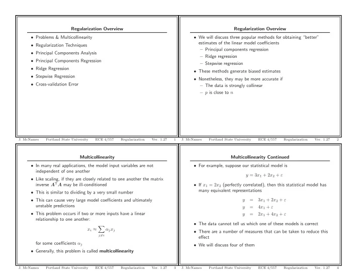
Regularization Overview Regularization Overview Problems & - PowerPoint PPT Presentation

Regularization Overview Regularization Overview • Problems & Multicollinearity • We will discuss three popular methods for obtaining “better” estimates of the linear model coefficients • Regularization Techniques – Principal components regression • Principal Components Analysis – Ridge regression • Principal Components Regression – Stepwise regression • Ridge Regression • These methods generate biased estimates • Stepwise Regression • Nonetheless, they may be more accurate if • Cross-validation Error – The data is strongly collinear – p is close to n J. McNames Portland State University ECE 4/557 Regularization Ver. 1.27 1 J. McNames Portland State University ECE 4/557 Regularization Ver. 1.27 2 Multicollinearity Multicollinearity Continued • In many real applications, the model input variables are not • For example, suppose our statistical model is independent of one another y = 3 x 1 + 2 x 2 + ε • Like scaling, if they are closely related to one another the matrix inverse A T A may be ill-conditioned • If x 1 = 2 x 2 (perfectly correlated), then this statistical model has many equivalent representations • This is similar to dividing by a very small number y = 3 x 1 + 2 x 2 + ε • This can cause very large model coefficients and ultimately unstable predictions y = 4 x 1 + ε • This problem occurs if two or more inputs have a linear y = 2 x 1 + 4 x 2 + ε relationship to one another: • The data cannot tell us which one of these models is correct � x i ≈ α j x j • There are a number of measures that can be taken to reduce this j � = i effect for some coefficients α j • We will discuss four of them • Generally, this problem is called multicollinearity J. McNames Portland State University ECE 4/557 Regularization Ver. 1.27 3 J. McNames Portland State University ECE 4/557 Regularization Ver. 1.27 4

Example 1: Multicollinearity Singular Value Decomposition n × p V T N = 20; n × p = U A Σ x1 = rand(N,1); n × n p × p x2 = 5*x1; om = [-1 2 3]’; % True process coefficients • The A matrix can be decomposed as a product of three different matrices A = [ones(N,1) x1 x2]; y = A*om + 0.1*randn(N,1); % Statistical model • U and V are unitary matrices b = y; w = inv(A’*A)*A’*b % Regression model coefficients U T U = I n × n = UU T V T V = I p × p = V V T • Σ is a diagonal matrix This returns ⎡ 0 0 ⎤ σ 1 . . . Warning: Matrix is close to singular or badly scaled. Results may be inaccurate. RCOND = 3.801412e-018. 0 σ 2 . . . 0 > In Multicollinearity at 11 ⎢ ⎥ ⎢ . . . ⎥ ... . . . ⎢ ⎥ . . . w = ⎢ ⎥ � � Σ + -1.0088 ⎢ ⎥ n × p = 0 0 = Σ . . . σ p ⎢ ⎥ 0 31.8756 ⎢ ⎥ 0 0 . . . 0 -1.0408 ⎢ ⎥ . . . ⎢ ... ⎥ . . . ⎢ ⎥ . . . ⎣ ⎦ 0 0 . . . 0 J. McNames Portland State University ECE 4/557 Regularization Ver. 1.27 5 J. McNames Portland State University ECE 4/557 Regularization Ver. 1.27 6 Singular Value Decomposition Continued 1 Singular Value Decomposition & PCA V T • The matrix U can be written as n × p = U + A Σ + p × p n × p p × p � � • The V matrix can be written in terms of its column vectors U = U + U − n × p n × ( n − p ) ⎡ ⎤ | | | p × p = V v 1 v 2 . . . v p • This enables us to decompose the A matrix slightly differently ⎣ ⎦ | | | n × p V T V T n × p = U p × p = U + A Σ Σ + • The square of the singular values ( σ 2 n × n p × p i ) represents the 2nd moment n × p p × p of the data along projections of A onto the vectors v i • The elements along the diagonal of Σ + are called the singular • The input vectors are rotated to the directions that maximize the values of A estimated second moment of the projected data • They are nonnegative || Av 1 || 2 = ( Av 1 ) T ( Av 1 ) = v 1 A T Av 1 v 1 = argmax • Usually they are ordered such that v T 1 v 1 =1 σ 1 ≥ σ 2 ≥ σ 3 ≥ · · · ≥ σ p ≥ 0 • Locating these vectors and their projected variances is called principal components analysis J. McNames Portland State University ECE 4/557 Regularization Ver. 1.27 7 J. McNames Portland State University ECE 4/557 Regularization Ver. 1.27 8

Example 2: PCA without Centering Example 2: MATLAB Code Principal Components Analysis Without Centering function [] = PCACentering (); %clear; 0.9 rand(’state ’ ,8); 0.8 randn(’state ’ ,11); 0.7 NP = 100; % Number of points x1 = 0.08*randn(NP ,1); % Input 1 0.6 x2 = -x1 + 0.04*randn(NP ,1); % Input 2 x1 = x1 + .5; 0.5 x2 = x2 + .5; x 2 0.4 A = [x1 x2 ones(NP ,1)]; [U,S,V] = svd(A); % Singular Value Decomposition 0.3 V(: ,1) = -V(: ,1); 0.2 figure; FigureSet (1 ,5 ,5); 0.1 ax = axes(’Position ’ ,[0.1 0.1 0.8 0.8 ]); h = plot(x1 ,x2 ,’r.’); set(h,’MarkerSize ’ ,6); 0 hold on; xlim ([-0.10 1.00 ]); −0.1 ylim ([-0.10 1.00 ]); −0.1 0 0.1 0.2 0.3 0.4 0.5 0.6 0.7 0.8 0.9 x 1 AxisLines; % Function in my collection J. McNames Portland State University ECE 4/557 Regularization Ver. 1.27 9 J. McNames Portland State University ECE 4/557 Regularization Ver. 1.27 10 p1 = [0 0]; % Starting point p1 = xc; p2 = V(1:2 ,1)*S(1 ,1)/15; % Ending point p2 = xc + V(: ,1)*S(1 ,1)/2; h = DrawArrow ([p1 (1) p2 (1)] ,[ p1 (2) p2 (2)]); % Function in my collection h = DrawArrow ([p1 (1) p2 (1)] ,[ p1 (2) p2 (2)]); set(h,’HeadStyle ’,’plain ’); set(h,’HeadStyle ’,’plain ’); p1 = [0 0]; p1 = xc; p2 = V(1:2 ,2)*S(2 ,2)/15; p2 = xc + V(: ,2)*S(2 ,2)/2; h = DrawArrow ([p1 (1) p2 (1)] ,[ p1 (2) p2 (2)]); h = DrawArrow ([p1 (1) p2 (1)] ,[ p1 (2) p2 (2)]); set(h,’HeadStyle ’,’plain ’); set(h,’HeadStyle ’,’plain ’); hold off; hold off; xlabel(’x_1 ’); axis(’square ’); ylabel(’x_2 ’); xlabel(’x_1 ’); title(’Principal Components Analysis Without Centering ’); ylabel(’x_2 ’); AxisSet (8); title(’Principal Components Analysis With Centering ’); print -depsc PCAUncentered.eps ; AxisSet (8); print -depsc PCACentered.eps ; x1c = mean(x1); % Find the average ( center) of x1 x2c = mean(x2); % Find the average ( center) of x2 xc = [x1c x2c]’; % Collect into a vector A = [x1 -x1c x2 -x2c ]; % Recreate the A matrix [U,S,V] = svd(A); figure; FigureSet (1 ,5 ,5); ax = axes(’Position ’ ,[0.1 0.1 0.8 0.8 ]); h = plot(x1 ,x2 ,’r.’); set(h,’MarkerSize ’ ,6); hold on; xlim ([-0.10 1.00 ]); ylim ([-0.10 1.00 ]); AxisLines; J. McNames Portland State University ECE 4/557 Regularization Ver. 1.27 11 J. McNames Portland State University ECE 4/557 Regularization Ver. 1.27 12

Principal Components Analysis Example 3: PCA With Centering • In general, finding the directions of maximum variance is more Principal Components Analysis With Centering useful than finding the directions that maximize the second 0.9 moment 0.8 • This can be achieved by subtracting the average from all of the input vectors 0.7 ⎡ ⎤ | | | 0.6 A ′ x ′ x ′ x ′ n × ( p − 1) = . . . 1 2 p − 1 0.5 ⎣ ⎦ x 2 | | | 0.4 where x ′ i = x i − ¯ x i 0.3 • If A ′ is decomposed as A ′ = U + Σ + V T , then 0.2 σ 2 σ 2 1 = var( Av 1 ) 2 = var( Av 2 ) . . . 0.1 0 • Note that the column of ones is omitted from A ′ −0.1 • The vectors v i now represent the directions of maximum variance −0.1 0 0.1 0.2 0.3 0.4 0.5 0.6 0.7 0.8 0.9 x 1 J. McNames Portland State University ECE 4/557 Regularization Ver. 1.27 13 J. McNames Portland State University ECE 4/557 Regularization Ver. 1.27 14 PCA & SVD PCA & SVD Summary A = U + Σ + V T A T A = V T Λ V A = U + Σ + V T A T A = V T Λ V p p • Often PCA is calculated using eigenvalues and eigenvectors � � u i σ i v T u i v T � � A = i = σ i i instead of singular value decomposition i =1 i =1 • It can be shown that • A can be expressed as a sum of p rank-1 matrices A T A = V T Λ V • PCA is useful for compression where ⎡ ⎤ λ 1 0 . . . 0 • If most of the variance is captured by the first few principal 0 λ 2 . . . 0 ⎢ ⎥ components, then we can omit the other components with p × p = Λ ⎢ . . ⎥ ... . . ⎢ ⎥ minimal loss of information . . 0 ⎣ ⎦ 0 0 . . . λ p • Just truncate the sum to get an approximation of A • This is the same V matrix as computed using SVD on A ρ � u i v T � � A ≈ σ i • The eigenvalues are related to the singular values by λ i = σ 2 i i i =1 for some ρ < p J. McNames Portland State University ECE 4/557 Regularization Ver. 1.27 15 J. McNames Portland State University ECE 4/557 Regularization Ver. 1.27 16