Reduced Basis Methods Karsten Urban for (some particular) Ulm - - PowerPoint PPT Presentation

reduced basis methods
SMART_READER_LITE
LIVE PREVIEW

Reduced Basis Methods Karsten Urban for (some particular) Ulm - - PowerPoint PPT Presentation

Reduced Basis Methods Karsten Urban for (some particular) Ulm University (Germany) HJB equations Institute for Numerical Mathematics page 1/27 RBM for HJB | RICAM 2016 | Karsten Urban | Acknowledgements Acknowledgements joint work with


slide-1
SLIDE 1

Karsten Urban

Ulm University (Germany) Institute for Numerical Mathematics

Reduced Basis Methods for (some particular) HJB equations

slide-2
SLIDE 2

page 1/27 RBM for HJB | RICAM 2016 | Karsten Urban | Acknowledgements

Acknowledgements

◮ joint work with

◮ R¨

udiger Kiesel (Duisburg-Essen)

◮ Silke Glas, Sebastian Steck (Ulm)

◮ Funding:

◮ Deutsche Forschungsgemeinschaft (DFG: GrK1100, Ur-63/9, SPP1324) ◮ Federal Ministry of Economy (BMWT)

slide-3
SLIDE 3

page 2/27 RBM for HJB | RICAM 2016 | Karsten Urban | Acknowledgements

Outline

1 “Particular”HJB: The EU-ETS 2

(A very short) Introduction to RBM

3

RBM for the EU-ETS-HJB

4

Conclusions and outlook

slide-4
SLIDE 4

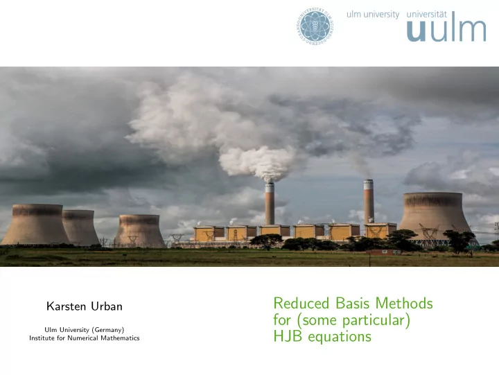
page 3/27 RBM for HJB | RICAM 2016 | Karsten Urban | “Particular” HJB: The EU-ETS

1 “Particular”HJB: The EU-ETS 2

(A very short) Introduction to RBM

3

RBM for the EU-ETS-HJB

4

Conclusions and outlook

slide-5
SLIDE 5

page 4/27 RBM for HJB | RICAM 2016 | Karsten Urban | “Particular” HJB: The EU-ETS

EU-ETS: European Union Emission Trading System

◮ anthropogenic global warming ◮ Kyoto protocol: limit of CO2-emissions ◮ according amount of emission permits are issued

slide-6
SLIDE 6

page 4/27 RBM for HJB | RICAM 2016 | Karsten Urban | “Particular” HJB: The EU-ETS

EU-ETS: European Union Emission Trading System

◮ anthropogenic global warming ◮ Kyoto protocol: limit of CO2-emissions ◮ according amount of emission permits are issued ◮ permits are traded at the exchange: EU-ETS ◮ penalty for emissions not covered by permits

slide-7
SLIDE 7

page 4/27 RBM for HJB | RICAM 2016 | Karsten Urban | “Particular” HJB: The EU-ETS

EU-ETS: European Union Emission Trading System

◮ anthropogenic global warming ◮ Kyoto protocol: limit of CO2-emissions ◮ according amount of emission permits are issued ◮ permits are traded at the exchange: EU-ETS ◮ penalty for emissions not covered by permits ◮ goal here: public control of EU-ETS: abate 5% of emissions

slide-8
SLIDE 8

page 5/27 RBM for HJB | RICAM 2016 | Karsten Urban | Model of the Emission Trading System

Modeling EU-ETS

◮ trading periods: [0, T] ◮ equlibirium ≡ sum of costs of all market participants is minimal[1]

[1]Camora, Fehr, Hinz: Optimal Stochastic Control and Carbon Price Formation, 2009

slide-9
SLIDE 9

page 5/27 RBM for HJB | RICAM 2016 | Karsten Urban | Model of the Emission Trading System

Modeling EU-ETS

◮ trading periods: [0, T] ◮ equlibirium ≡ sum of costs of all market participants is minimal[1] ◮ state Yτ ∈ Rd, τ ∈ [0, T]: amount of uncovered emissions (d: # companies)

[1]Camora, Fehr, Hinz: Optimal Stochastic Control and Carbon Price Formation, 2009

slide-10
SLIDE 10

page 5/27 RBM for HJB | RICAM 2016 | Karsten Urban | Model of the Emission Trading System

Modeling EU-ETS

◮ trading periods: [0, T] ◮ equlibirium ≡ sum of costs of all market participants is minimal[1] ◮ state Yτ ∈ Rd, τ ∈ [0, T]: amount of uncovered emissions (d: # companies) ◮ control πτ ∈ Rd: additional abatement compared to business as usual

[1]Camora, Fehr, Hinz: Optimal Stochastic Control and Carbon Price Formation, 2009

slide-11
SLIDE 11

page 5/27 RBM for HJB | RICAM 2016 | Karsten Urban | Model of the Emission Trading System

Modeling EU-ETS

◮ trading periods: [0, T] ◮ equlibirium ≡ sum of costs of all market participants is minimal[1] ◮ state Yτ ∈ Rd, τ ∈ [0, T]: amount of uncovered emissions (d: # companies) ◮ control πτ ∈ Rd: additional abatement compared to business as usual ◮ optimal abatement strategy π = (πτ)τ∈[0,T]:

should minimize the expected abatement costs (cost functional) J(π) := E T f π (τ, Yτ) dτ + h(YT)

  • ◮ f π: running abatement cost using strategy π

◮ h: penalty at the end of the trading period

[1]Camora, Fehr, Hinz: Optimal Stochastic Control and Carbon Price Formation, 2009

slide-12
SLIDE 12

page 5/27 RBM for HJB | RICAM 2016 | Karsten Urban | Model of the Emission Trading System

Modeling EU-ETS

◮ trading periods: [0, T] ◮ equlibirium ≡ sum of costs of all market participants is minimal[1] ◮ state Yτ ∈ Rd, τ ∈ [0, T]: amount of uncovered emissions (d: # companies) ◮ control πτ ∈ Rd: additional abatement compared to business as usual ◮ optimal abatement strategy π = (πτ)τ∈[0,T]:

should minimize the expected abatement costs (cost functional) J(π) := E T f π (τ, Yτ) dτ + h(YT)

  • ◮ f π: running abatement cost using strategy π

◮ h: penalty at the end of the trading period

◮ stochastic model for Yτ:

dYτ = bπ(τ, Yτ)dτ + σπ(τ, Yτ)dWτ, τ ∈ (0, T], Y0 = y0

◮ Wτ: a d-dimensional Wiener process ◮ bπ, σπ: drift and volatility coefficients, bπ, σπ(σπ)T linear in π.

[1]Camora, Fehr, Hinz: Optimal Stochastic Control and Carbon Price Formation, 2009

slide-13
SLIDE 13

page 5/27 RBM for HJB | RICAM 2016 | Karsten Urban | Model of the Emission Trading System

Modeling EU-ETS

◮ trading periods: [0, T] ◮ equlibirium ≡ sum of costs of all market participants is minimal[1] ◮ state Yτ ∈ Rd, τ ∈ [0, T]: amount of uncovered emissions (d: # companies) ◮ control πτ ∈ Rd: additional abatement compared to business as usual ◮ optimal abatement strategy π = (πτ)τ∈[0,T]:

should minimize the expected abatement costs (cost functional) J(t, x; γ) := E T

t

f γ (τ, Yτ) dτ + h(YT)

  • ◮ f π: running abatement cost using strategy π

◮ h: penalty at the end of the trading period

◮ stochastic model for Yτ:

dYτ = bπ(τ, Yτ)dτ + σπ(τ, Yτ)dWτ, τ ∈ (t, T], Yt = x

◮ Wτ: a d-dimensional Wiener process ◮ bπ, σπ: drift and volatility coefficients, bπ, σπ(σπ)T linear in π.

[1]Camora, Fehr, Hinz: Optimal Stochastic Control and Carbon Price Formation, 2009

slide-14
SLIDE 14

page 6/27 RBM for HJB | RICAM 2016 | Karsten Urban | Model of the Emission Trading System

(Parameterized) Hamilton Jacobi Bellman Equation 1/3

◮ value function (x ∈ Rd)

u(t, x) = inf

γ∈Γ J(t, x; γ)

∀t ∈ [0, T), u(T, x) = h(x)

◮ Γ ⊂ L∞((0, T) × Rd; Rd): set of admissible controls

[2]Yong, Zhou: Stochastic controls: Hamiltonian systems and HJB equations, 1999

slide-15
SLIDE 15

page 6/27 RBM for HJB | RICAM 2016 | Karsten Urban | Model of the Emission Trading System

(Parameterized) Hamilton Jacobi Bellman Equation 1/3

◮ value function (x ∈ Rd)

u(t, x) = inf

γ∈Γ J(t, x; γ)

∀t ∈ [0, T), u(T, x) = h(x)

◮ Γ ⊂ L∞((0, T) × Rd; Rd): set of admissible controls ◮ HJB[2]

∂tu(t, x) + sup

γ∈Γ

1 2tr(σγ(σγ)T ∇2u(t, x)) + bγ · ∇u(t, x) − f γ(t, x)

  • = 0

[2]Yong, Zhou: Stochastic controls: Hamiltonian systems and HJB equations, 1999

slide-16
SLIDE 16

page 6/27 RBM for HJB | RICAM 2016 | Karsten Urban | Model of the Emission Trading System

(Parameterized) Hamilton Jacobi Bellman Equation 1/3

◮ value function (x ∈ Rd)

u(t, x) = inf

γ∈Γ J(t, x; γ)

∀t ∈ [0, T), u(T, x) = h(x)

◮ Γ ⊂ L∞((0, T) × Rd; Rd): set of admissible controls ◮ HJB[2]

∂tu(t, x) + sup

γ∈Γ

1 2tr(σγ(σγ)T ∇2u(t, x)) + bγ · ∇u(t, x) − f γ(t, x)

  • = 0

◮ parameters µ ∈ D ⊂ RP

e.g. regulatory constraints, market values, etc. f γ(µ), bγ(µ), σγ(µ), J(µ; t, x; γ) u(µ) = u(µ; t, x)

[2]Yong, Zhou: Stochastic controls: Hamiltonian systems and HJB equations, 1999

slide-17
SLIDE 17

page 6/27 RBM for HJB | RICAM 2016 | Karsten Urban | Model of the Emission Trading System

(Parameterized) Hamilton Jacobi Bellman Equation 1/3

◮ value function (x ∈ Rd)

u(t, x) = inf

γ∈Γ J(t, x; γ)

∀t ∈ [0, T), u(T, x) = h(x)

◮ Γ ⊂ L∞((0, T) × Rd; Rd): set of admissible controls ◮ HJB[2]

∂tu(t, x) + sup

γ∈Γ

1 2tr(σγ(σγ)T ∇2u(t, x)) + bγ · ∇u(t, x) − f γ(t, x)

  • = 0

◮ parameters µ ∈ D ⊂ RP

e.g. regulatory constraints, market values, etc. f γ(µ), bγ(µ), σγ(µ), J(µ; t, x; γ) u(µ) = u(µ; t, x)

◮ Goal: find“optimal”parameters (also in realtime)

[2]Yong, Zhou: Stochastic controls: Hamiltonian systems and HJB equations, 1999

slide-18
SLIDE 18

page 7/27 RBM for HJB | RICAM 2016 | Karsten Urban | Model of the Emission Trading System

(Parameterized) Hamilton Jacobi Bellman Equation 2/3

◮ parameterized coefficients:

u → Aγ(µ; u) := −aγ(µ) ∆u + bγ(µ) · ∇u + cγ(µ)u, µ ∈ D.

slide-19
SLIDE 19

page 7/27 RBM for HJB | RICAM 2016 | Karsten Urban | Model of the Emission Trading System

(Parameterized) Hamilton Jacobi Bellman Equation 2/3

◮ parameterized coefficients:

u → Aγ(µ; u) := −aγ(µ) ∆u + bγ(µ) · ∇u + cγ(µ)u, µ ∈ D.

◮ parameterized Hamilton-type operator

H(µ; u) := sup

γ∈Γ

{Aγ(µ; u) − f γ(µ)}

slide-20
SLIDE 20

page 7/27 RBM for HJB | RICAM 2016 | Karsten Urban | Model of the Emission Trading System

(Parameterized) Hamilton Jacobi Bellman Equation 2/3

◮ parameterized coefficients:

u → Aγ(µ; u) := −aγ(µ) ∆u + bγ(µ) · ∇u + cγ(µ)u, µ ∈ D.

◮ parameterized Hamilton-type operator

H(µ; u) := sup

γ∈Γ

{Aγ(µ; u) − f γ(µ)}

◮ P-HJB

∂tu + H(µ; u) = 0, in ΩT, (1a) ∂ ∂nu = ψ,

  • n ∂ΩT = (0, T) × ∂Ω,

(1b) u(T) = uT,

  • n ¯

Ω, (1c)

slide-21
SLIDE 21

page 8/27 RBM for HJB | RICAM 2016 | Karsten Urban | Model of the Emission Trading System

(Parameterized) Hamilton Jacobi Bellman Equation 3/3

◮ parameterized (linear) space-time differential operator

Lγ(µ; u) := ∂tu + Aγ(µ; u)

slide-22
SLIDE 22

page 8/27 RBM for HJB | RICAM 2016 | Karsten Urban | Model of the Emission Trading System

(Parameterized) Hamilton Jacobi Bellman Equation 3/3

◮ parameterized (linear) space-time differential operator

Lγ(µ; u) := ∂tu + Aγ(µ; u)

◮ P-HJB revisited

sup

γ∈Γ

{Lγ(µ; u) − g γ(µ)} = 0

  • n ΩT

u∗ = u∗(µ) ∈ U (solution space)

slide-23
SLIDE 23

page 8/27 RBM for HJB | RICAM 2016 | Karsten Urban | Model of the Emission Trading System

(Parameterized) Hamilton Jacobi Bellman Equation 3/3

◮ parameterized (linear) space-time differential operator

Lγ(µ; u) := ∂tu + Aγ(µ; u)

◮ P-HJB revisited

sup

γ∈Γ

{Lγ(µ; u) − g γ(µ)} = 0

  • n ΩT

u∗ = u∗(µ) ∈ U (solution space)

◮ optimal (parameter-dependent) control

Γ ∋ γ∗(µ) = arg sup

γ∈Γ

{Lγ(µ; u∗) − g γ(µ)}

◮ couple x∗ = x∗(µ) = (γ∗(µ), u∗(µ)) ∈ Γ × U

slide-24
SLIDE 24

page 8/27 RBM for HJB | RICAM 2016 | Karsten Urban | Model of the Emission Trading System

(Parameterized) Hamilton Jacobi Bellman Equation 3/3

◮ parameterized (linear) space-time differential operator

Lγ(µ; u) := ∂tu + Aγ(µ; u)

◮ P-HJB revisited

sup

γ∈Γ

{Lγ(µ; u) − g γ(µ)} = 0

  • n ΩT

u∗ = u∗(µ) ∈ U (solution space)

◮ optimal (parameter-dependent) control

Γ ∋ γ∗(µ) = arg sup

γ∈Γ

{Lγ(µ; u∗) − g γ(µ)}

◮ couple x∗ = x∗(µ) = (γ∗(µ), u∗(µ)) ∈ Γ × U ◮ Goal: determine x∗(µ) for many values of µ in realtime

slide-25
SLIDE 25

page 9/27 RBM for HJB | RICAM 2016 | Karsten Urban | (A very short) Introduction to RBM

1 “Particular”HJB: The EU-ETS 2

(A very short) Introduction to RBM

3

RBM for the EU-ETS-HJB

4

Conclusions and outlook

slide-26
SLIDE 26

page 10/27 RBM for HJB | RICAM 2016 | Karsten Urban | (A very short) Introduction to RBM

(A very short) Introduction to RBM

◮ 1st application: Thermal Fin

(∼ 2000, Patera, Maday, et al.)

◮ variable length of ribs

(∼ parameter)

◮ goal: optimization

◮ w.r.t. desired heat conduction ◮ for fixed volume ◮ with size constraints Picture courtesy of A.T. Patera, D.V. Rovas and L. Machiels, 2000

slide-27
SLIDE 27

page 10/27 RBM for HJB | RICAM 2016 | Karsten Urban | (A very short) Introduction to RBM

(A very short) Introduction to RBM

◮ 1st application: Thermal Fin

(∼ 2000, Patera, Maday, et al.)

◮ variable length of ribs

(∼ parameter)

◮ goal: optimization

◮ w.r.t. desired heat conduction ◮ for fixed volume ◮ with size constraints Picture courtesy of A.T. Patera, D.V. Rovas and L. Machiels, 2000

Mathematical Model: Parameterized PDE (PPDE) – linear

◮ µ ∈ D ⊂ RP: parameter; Ω ⊂ Rd: (spatial) domain for the pde

slide-28
SLIDE 28

page 10/27 RBM for HJB | RICAM 2016 | Karsten Urban | (A very short) Introduction to RBM

(A very short) Introduction to RBM

◮ 1st application: Thermal Fin

(∼ 2000, Patera, Maday, et al.)

◮ variable length of ribs

(∼ parameter)

◮ goal: optimization

◮ w.r.t. desired heat conduction ◮ for fixed volume ◮ with size constraints Picture courtesy of A.T. Patera, D.V. Rovas and L. Machiels, 2000

Mathematical Model: Parameterized PDE (PPDE) – linear

◮ µ ∈ D ⊂ RP: parameter; Ω ⊂ Rd: (spatial) domain for the pde ◮ X := X(Ω), Y := Y (Ω): function spaces (Sobolev space with BCs)

slide-29
SLIDE 29

page 10/27 RBM for HJB | RICAM 2016 | Karsten Urban | (A very short) Introduction to RBM

(A very short) Introduction to RBM

◮ 1st application: Thermal Fin

(∼ 2000, Patera, Maday, et al.)

◮ variable length of ribs

(∼ parameter)

◮ goal: optimization

◮ w.r.t. desired heat conduction ◮ for fixed volume ◮ with size constraints Picture courtesy of A.T. Patera, D.V. Rovas and L. Machiels, 2000

Mathematical Model: Parameterized PDE (PPDE) – linear

◮ µ ∈ D ⊂ RP: parameter; Ω ⊂ Rd: (spatial) domain for the pde ◮ X := X(Ω), Y := Y (Ω): function spaces (Sobolev space with BCs) ◮ A : X × Y × D: parametric form (often bilinear in 1st and 2nd argument)

slide-30
SLIDE 30

page 10/27 RBM for HJB | RICAM 2016 | Karsten Urban | (A very short) Introduction to RBM

(A very short) Introduction to RBM

◮ 1st application: Thermal Fin

(∼ 2000, Patera, Maday, et al.)

◮ variable length of ribs

(∼ parameter)

◮ goal: optimization

◮ w.r.t. desired heat conduction ◮ for fixed volume ◮ with size constraints Picture courtesy of A.T. Patera, D.V. Rovas and L. Machiels, 2000

Mathematical Model: Parameterized PDE (PPDE) – linear

◮ µ ∈ D ⊂ RP: parameter; Ω ⊂ Rd: (spatial) domain for the pde ◮ X := X(Ω), Y := Y (Ω): function spaces (Sobolev space with BCs) ◮ A : X × Y × D: parametric form (often bilinear in 1st and 2nd argument) ◮

seek u(µ) ∈ X: A(u(µ), w; µ) = 0 ∀w ∈ Y (PPDE for many µ)

slide-31
SLIDE 31

page 10/27 RBM for HJB | RICAM 2016 | Karsten Urban | (A very short) Introduction to RBM

(A very short) Introduction to RBM

◮ 1st application: Thermal Fin

(∼ 2000, Patera, Maday, et al.)

◮ variable length of ribs

(∼ parameter)

◮ goal: optimization

◮ w.r.t. desired heat conduction ◮ for fixed volume ◮ with size constraints Picture courtesy of A.T. Patera, D.V. Rovas and L. Machiels, 2000

Mathematical Model: Parameterized PDE (PPDE) – linear

◮ µ ∈ D ⊂ RP: parameter; Ω ⊂ Rd: (spatial) domain for the pde ◮ X := X(Ω), Y := Y (Ω): function spaces (Sobolev space with BCs) ◮ A : X × Y × D: parametric form (often bilinear in 1st and 2nd argument) ◮

seek u(µ) ∈ X: A(u(µ), w; µ) = 0 ∀w ∈ Y (PPDE for many µ)

◮ Output: s(µ) := ℓ(u(µ)), ℓ : X → R

slide-32
SLIDE 32

page 11/27 RBM for HJB | RICAM 2016 | Karsten Urban | (A very short) Introduction to RBM

(A very short) Introduction to RBM PPDE

◮ u(µ) ∈ X: A(u(µ), w; µ) = 0 ∀w ∈ Y (PPDE) ◮ Output: s(µ) := ℓ(u(µ))

Common situation / observation / assumption

◮ PPDE must be solved for many parameters µ: many-query (like optimization)

slide-33
SLIDE 33

page 11/27 RBM for HJB | RICAM 2016 | Karsten Urban | (A very short) Introduction to RBM

(A very short) Introduction to RBM PPDE

◮ u(µ) ∈ X: A(u(µ), w; µ) = 0 ∀w ∈ Y (PPDE) ◮ Output: s(µ) := ℓ(u(µ))

Common situation / observation / assumption

◮ PPDE must be solved for many parameters µ: many-query (like optimization) ◮ u(µ) (often) depends smoothly on µ ◮ detailed discretization X N , Y N , dim(X N ) = dim(Y N ) = N large;

uN ≈ u indistinguishable (‘truth’)

slide-34
SLIDE 34

page 12/27 RBM for HJB | RICAM 2016 | Karsten Urban | (A very short) Introduction to RBM

Introduction to RBM ‘Good’ RBM situation / Idea for RBM

◮ offline/online-decomposition possible:

slide-35
SLIDE 35

page 12/27 RBM for HJB | RICAM 2016 | Karsten Urban | (A very short) Introduction to RBM

Introduction to RBM ‘Good’ RBM situation / Idea for RBM

◮ offline/online-decomposition possible:

◮ offline: pre-compute“snapshots”uN (µi) = u(µi), i = 1, . . . , N for certain µi

(by e.g. FEM) – choice by error estimate

uN(µnew) =? {uN(µ)} uN(µ3) uN(µ2) uN(µ1)

◮ Form a reduced basis out of N

solutions uN (µ1), . . . , uN (µN)

  • ffline
slide-36
SLIDE 36

page 12/27 RBM for HJB | RICAM 2016 | Karsten Urban | (A very short) Introduction to RBM

Introduction to RBM ‘Good’ RBM situation / Idea for RBM

◮ offline/online-decomposition possible:

◮ offline: pre-compute“snapshots”uN (µi) = u(µi), i = 1, . . . , N for certain µi

(by e.g. FEM) – choice by error estimate

◮ online: for new µ ∈ {µi : i = 1, . . . , N} compute (Petrov-)Galerkin projection

uN(µ) ≈ u(µ) onto XN := span{uN (µi) : i = 1, . . . , N} (RB approx.)

uN(µnew) =? {uN(µ)} uN(µ3) uN(µ2) uN(µ1)

◮ Form a reduced basis out of N

solutions uN (µ1), . . . , uN (µN)

  • ffline
slide-37
SLIDE 37

page 12/27 RBM for HJB | RICAM 2016 | Karsten Urban | (A very short) Introduction to RBM

Introduction to RBM ‘Good’ RBM situation / Idea for RBM

◮ offline/online-decomposition possible:

◮ offline: pre-compute“snapshots”uN (µi) = u(µi), i = 1, . . . , N for certain µi

(by e.g. FEM) – choice by error estimate

◮ online: for new µ ∈ {µi : i = 1, . . . , N} compute (Petrov-)Galerkin projection

uN(µ) ≈ u(µ) onto XN := span{uN (µi) : i = 1, . . . , N} (RB approx.)

◮ in some cases (or you have to assume/numerically check it):

◮ uN (µ) − uN(µ) e−αN (rapid decay) N ≪ N suffices ◮ online complexity independent of N (

“online efficient” )

uN(µnew) =? {uN(µ)} uN(µ3) uN(µ2) uN(µ1)

◮ Form a reduced basis out of N

solutions uN (µ1), . . . , uN (µN)

  • ffline
slide-38
SLIDE 38

page 13/27 RBM for HJB | RICAM 2016 | Karsten Urban | (A very short) Introduction to RBM

When to use RBM ... and when not Consequences

◮ RB-approximation can only be as good as truth approximation

slide-39
SLIDE 39

page 13/27 RBM for HJB | RICAM 2016 | Karsten Urban | (A very short) Introduction to RBM

When to use RBM ... and when not Consequences

◮ RB-approximation can only be as good as truth approximation ◮ Benchmark: Kolmogorov N-width (1936) (for S ⊂ X)

dN(S) := inf

XN⊂X N ; dim(XN)=N

sup

uN ∈S

sup

uN∈XN

uN − uN

Buffa, Maday, Patera,Haasdonk, Cohen, Dahmen, DeVore, ...

slide-40
SLIDE 40

page 13/27 RBM for HJB | RICAM 2016 | Karsten Urban | (A very short) Introduction to RBM

When to use RBM ... and when not Consequences

◮ RB-approximation can only be as good as truth approximation ◮ Benchmark: Kolmogorov N-width (1936) (for S ⊂ X)

dN(S) := inf

XN⊂X N ; dim(XN)=N

sup

uN ∈S

sup

uN∈XN

uN − uN

Buffa, Maday, Patera,Haasdonk, Cohen, Dahmen, DeVore, ...

◮ complexity-offset by offline phase RBM (only) reasonable, if

◮ many evaluations required

(‘many-query context’)

◮ very fast or limited evaluations

required (‘realtime context’)

total complexity

  • ffline

complexity RBM direct solution for each µnew # new parameters µnew

slide-41
SLIDE 41

page 13/27 RBM for HJB | RICAM 2016 | Karsten Urban | (A very short) Introduction to RBM

When to use RBM ... and when not Consequences

◮ RB-approximation can only be as good as truth approximation ◮ Benchmark: Kolmogorov N-width (1936) (for S ⊂ X)

dN(S) := inf

XN⊂X N ; dim(XN)=N

sup

uN ∈S

sup

uN∈XN

uN − uN

Buffa, Maday, Patera,Haasdonk, Cohen, Dahmen, DeVore, ...

◮ complexity-offset by offline phase RBM (only) reasonable, if

◮ many evaluations required

(‘many-query context’)

◮ very fast or limited evaluations

required (‘realtime context’)

Use the right tool!

slide-42
SLIDE 42

page 14/27 RBM for HJB | RICAM 2016 | Karsten Urban | (A very short) Introduction to RBM

RBM – A posteriori error analysis / how to compute an RB Well-posedness assumption for PPDE A(u(µ), w; µ) = 0 ∀w ∈ Y

◮ βLB := inf

µ∈D inf v∈X sup w∈Y

A(v, w; µ) > 0 ◮ γUB := sup

µ∈D

sup

v∈X

sup

w∈Y

A(v, w; µ) vX wY < ∞

slide-43
SLIDE 43

page 14/27 RBM for HJB | RICAM 2016 | Karsten Urban | (A very short) Introduction to RBM

RBM – A posteriori error analysis / how to compute an RB Well-posedness assumption for PPDE A(u(µ), w; µ) = 0 ∀w ∈ Y

◮ βLB := inf

µ∈D inf v∈X sup w∈Y

A(v, w; µ) > 0 ◮ γUB := sup

µ∈D

sup

v∈X

sup

w∈Y

A(v, w; µ) vX wY < ∞

◮ e.g.: A(w, v; µ) = b(w, v; µ) − f (µ), v

slide-44
SLIDE 44

page 14/27 RBM for HJB | RICAM 2016 | Karsten Urban | (A very short) Introduction to RBM

RBM – A posteriori error analysis / how to compute an RB Well-posedness assumption for PPDE A(u(µ), w; µ) = 0 ∀w ∈ Y

◮ βLB := inf

µ∈D inf v∈X sup w∈Y

A(v, w; µ) > 0 ◮ γUB := sup

µ∈D

sup

v∈X

sup

w∈Y

A(v, w; µ) vX wY < ∞

◮ e.g.: A(w, v; µ) = b(w, v; µ) − f (µ), v ◮ Exact error: eN(µ) := u(µ) − uN(µ); residual: rN(v; µ) := A(uN(µ), v; µ)

slide-45
SLIDE 45

page 15/27 RBM for HJB | RICAM 2016 | Karsten Urban | (A very short) Introduction to RBM

RBM – A posteriori error analysis

◮ e.g.: A(v, w; µ) = b(v, w; µ) − f (µ), v; ◮ Exact error: eN(µ) := u(µ) − uN(µ); residual: rN(w; µ) := A(uN(µ), v; µ)

slide-46
SLIDE 46

page 15/27 RBM for HJB | RICAM 2016 | Karsten Urban | (A very short) Introduction to RBM

RBM – A posteriori error analysis

◮ e.g.: A(v, w; µ) = b(v, w; µ) − f (µ), v; ◮ Exact error: eN(µ) := u(µ) − uN(µ); residual: rN(w; µ) := A(uN(µ), v; µ)

Thus:

◮ inf-sup and definition of dual norm:

eN(µ)X ≤

  • βLB

−1 sup

w∈Y

A(eN(µ), w; µ) wY =

  • βLB

−1 sup

w∈Y

A(uN(µ), w; µ) wY

slide-47
SLIDE 47

page 15/27 RBM for HJB | RICAM 2016 | Karsten Urban | (A very short) Introduction to RBM

RBM – A posteriori error analysis

◮ e.g.: A(v, w; µ) = b(v, w; µ) − f (µ), v; ◮ Exact error: eN(µ) := u(µ) − uN(µ); residual: rN(w; µ) := A(uN(µ), v; µ)

Thus:

◮ inf-sup and definition of dual norm:

eN(µ)X ≤

  • βLB

−1 sup

w∈Y

A(eN(µ), w; µ) wY =

  • βLB

−1 sup

w∈Y

A(uN(µ), w; µ) wY =

  • βLB

−1 rN(µ)Y ′ eN(µ)X ≤

  • βLB

−1 rN(µ)Y ′ =: ∆N(µ)

slide-48
SLIDE 48

page 15/27 RBM for HJB | RICAM 2016 | Karsten Urban | (A very short) Introduction to RBM

RBM – A posteriori error analysis

◮ e.g.: A(v, w; µ) = b(v, w; µ) − f (µ), v; ◮ Exact error: eN(µ) := u(µ) − uN(µ); residual: rN(w; µ) := A(uN(µ), v; µ)

Thus:

◮ inf-sup and definition of dual norm:

eN(µ)X ≤

  • βLB

−1 sup

w∈Y

A(eN(µ), w; µ) wY =

  • βLB

−1 sup

w∈Y

A(uN(µ), w; µ) wY =

  • βLB

−1 rN(µ)Y ′ eN(µ)X ≤

  • βLB

−1 rN(µ)Y ′ =: ∆N(µ) ⇒ ∆N(µ) should be efficiently computable and efficient! Compute sup

w∈Y

rN(w; µ) wY (wavelets; Ali, Steih, U., 2016) or use sup

w N ∈Y N

rN(w N ; µ) w N Y N

slide-49
SLIDE 49

page 16/27 RBM for HJB | RICAM 2016 | Karsten Urban | (A very short) Introduction to RBM

RB determination (offline)

◮ use error estimator ∆N(µ)

slide-50
SLIDE 50

page 16/27 RBM for HJB | RICAM 2016 | Karsten Urban | (A very short) Introduction to RBM

RB determination (offline)

◮ use error estimator ∆N(µ) ◮ maximize ∆N(µ) over finite µ ∈ Dtest

(Greedy: Patera, Maday et. al.; Nonlinear optimization: Ghattas et. al., Volkwein, U., Zeeb)

slide-51
SLIDE 51

page 16/27 RBM for HJB | RICAM 2016 | Karsten Urban | (A very short) Introduction to RBM

RB determination (offline)

◮ use error estimator ∆N(µ) ◮ maximize ∆N(µ) over finite µ ∈ Dtest

(Greedy: Patera, Maday et. al.; Nonlinear optimization: Ghattas et. al., Volkwein, U., Zeeb) parameters, snapshots, reduced spaces XN, YN

slide-52
SLIDE 52

page 16/27 RBM for HJB | RICAM 2016 | Karsten Urban | (A very short) Introduction to RBM

RB determination (offline)

◮ use error estimator ∆N(µ) ◮ maximize ∆N(µ) over finite µ ∈ Dtest

(Greedy: Patera, Maday et. al.; Nonlinear optimization: Ghattas et. al., Volkwein, U., Zeeb) parameters, snapshots, reduced spaces XN, YN

◮ precompute all µ-independent terms offline

(EIM: Maday et. al.) N-independent online stage

slide-53
SLIDE 53

page 16/27 RBM for HJB | RICAM 2016 | Karsten Urban | (A very short) Introduction to RBM

RB determination (offline)

◮ use error estimator ∆N(µ) ◮ maximize ∆N(µ) over finite µ ∈ Dtest

(Greedy: Patera, Maday et. al.; Nonlinear optimization: Ghattas et. al., Volkwein, U., Zeeb) parameters, snapshots, reduced spaces XN, YN

◮ precompute all µ-independent terms offline

(EIM: Maday et. al.) N-independent online stage

◮ online certification via ∆N(µ)

slide-54
SLIDE 54

page 16/27 RBM for HJB | RICAM 2016 | Karsten Urban | (A very short) Introduction to RBM

RB determination (offline)

◮ use error estimator ∆N(µ) ◮ maximize ∆N(µ) over finite µ ∈ Dtest

(Greedy: Patera, Maday et. al.; Nonlinear optimization: Ghattas et. al., Volkwein, U., Zeeb) parameters, snapshots, reduced spaces XN, YN

◮ precompute all µ-independent terms offline

(EIM: Maday et. al.) N-independent online stage

◮ online certification via ∆N(µ)

⇒ error estimate ∆N(µ) is crucial:

◮ sharpness ∼ N ◮ if residual based, we need to compute the inf-sup-constant

(e.g. SCM, Maday, Patera et. al.)

◮ instationary: POD-Greedy or space-time (Mayerhofer, Glas, U.)

slide-55
SLIDE 55

page 17/27 RBM for HJB | RICAM 2016 | Karsten Urban | RBM for the EU-ETS-HJB

1 “Particular”HJB: The EU-ETS 2

(A very short) Introduction to RBM

3

RBM for the EU-ETS-HJB

4

Conclusions and outlook

slide-56
SLIDE 56

page 18/27 RBM for HJB | RICAM 2016 | Karsten Urban | RBM for the EU-ETS-HJB

RBM for HJB — detailed ( “truth” ) discretization 1/2

◮ Z := {zi := (ti, xi) ∈ ΩT = (0, T) × Ω : i = 1, . . . , N}, N ≫ 1:

points in time-space

slide-57
SLIDE 57

page 18/27 RBM for HJB | RICAM 2016 | Karsten Urban | RBM for the EU-ETS-HJB

RBM for HJB — detailed ( “truth” ) discretization 1/2

◮ Z := {zi := (ti, xi) ∈ ΩT = (0, T) × Ω : i = 1, . . . , N}, N ≫ 1:

points in time-space

◮ u∗(µ) = (u∗ i (µ))i=1,...,N ∈ RN ≈ u∗(µ) on Z

slide-58
SLIDE 58

page 18/27 RBM for HJB | RICAM 2016 | Karsten Urban | RBM for the EU-ETS-HJB

RBM for HJB — detailed ( “truth” ) discretization 1/2

◮ Z := {zi := (ti, xi) ∈ ΩT = (0, T) × Ω : i = 1, . . . , N}, N ≫ 1:

points in time-space

◮ u∗(µ) = (u∗ i (µ))i=1,...,N ∈ RN ≈ u∗(µ) on Z

  • ptimization problems for each zi ∈ Z; result: γ∗

i (µ) ∈ Rd

slide-59
SLIDE 59

page 18/27 RBM for HJB | RICAM 2016 | Karsten Urban | RBM for the EU-ETS-HJB

RBM for HJB — detailed ( “truth” ) discretization 1/2

◮ Z := {zi := (ti, xi) ∈ ΩT = (0, T) × Ω : i = 1, . . . , N}, N ≫ 1:

points in time-space

◮ u∗(µ) = (u∗ i (µ))i=1,...,N ∈ RN ≈ u∗(µ) on Z

  • ptimization problems for each zi ∈ Z; result: γ∗

i (µ) ∈ Rd ◮ let Lγ Z ∈ RN×N , gγ Z ∈ RN : some discretization of Lγ, g γ on Z

(e.g. collocation, nodal interpolation, finite differences, ...)

slide-60
SLIDE 60

page 18/27 RBM for HJB | RICAM 2016 | Karsten Urban | RBM for the EU-ETS-HJB

RBM for HJB — detailed ( “truth” ) discretization 1/2

◮ Z := {zi := (ti, xi) ∈ ΩT = (0, T) × Ω : i = 1, . . . , N}, N ≫ 1:

points in time-space

◮ u∗(µ) = (u∗ i (µ))i=1,...,N ∈ RN ≈ u∗(µ) on Z

  • ptimization problems for each zi ∈ Z; result: γ∗

i (µ) ∈ Rd ◮ let Lγ Z ∈ RN×N , gγ Z ∈ RN : some discretization of Lγ, g γ on Z

(e.g. collocation, nodal interpolation, finite differences, ...)

◮ determine u∗(µ) ∈ RN by solving

Find u(µ) ∈ RN : max

γi∈Rd{Lγi Z (µ) u(µ) − gγi Z (µ)} = 0,

∀1 ≤ i ≤ N.

slide-61
SLIDE 61

page 18/27 RBM for HJB | RICAM 2016 | Karsten Urban | RBM for the EU-ETS-HJB

RBM for HJB — detailed ( “truth” ) discretization 1/2

◮ Z := {zi := (ti, xi) ∈ ΩT = (0, T) × Ω : i = 1, . . . , N}, N ≫ 1:

points in time-space

◮ u∗(µ) = (u∗ i (µ))i=1,...,N ∈ RN ≈ u∗(µ) on Z

  • ptimization problems for each zi ∈ Z; result: γ∗

i (µ) ∈ Rd ◮ let Lγ Z ∈ RN×N , gγ Z ∈ RN : some discretization of Lγ, g γ on Z

(e.g. collocation, nodal interpolation, finite differences, ...)

◮ determine u∗(µ) ∈ RN by solving

Find u(µ) ∈ RN : max

γi∈Rd{Lγi Z (µ) u(µ) − gγi Z (µ)} = 0,

∀1 ≤ i ≤ N.

◮ find optimal control by:

Rd ∋ γ∗

i (µ) := arg max γi∈Rd{Lγi Z (µ)u(µ) − gγi Z (µ)},

1 ≤ i ≤ N.

slide-62
SLIDE 62

page 19/27 RBM for HJB | RICAM 2016 | Karsten Urban | RBM for the EU-ETS-HJB

RB - detailed ( “truth” ) discretization 2/2

◮ write this as one large system:

Lγ∗ (µ) u∗(µ) − gγ∗ (µ) = 0 in RN ∂γ[Lγ∗(µ)u∗(µ) − gγ∗(µ)](δ) = 0, ∀δ ∈ RN×d

slide-63
SLIDE 63

page 19/27 RBM for HJB | RICAM 2016 | Karsten Urban | RBM for the EU-ETS-HJB

RB - detailed ( “truth” ) discretization 2/2

◮ write this as one large system:

Lγ∗ (µ) u∗(µ) − gγ∗ (µ) = 0 in RN ∂γ[Lγ∗(µ)u∗(µ) − gγ∗(µ)](δ) = 0, ∀δ ∈ RN×d

◮ or, as one system

0 = G(x; µ) :=  ∂γ[Lγ(µ) u(µ) − gγ(µ)] Lγ(µ)u(µ) − gγ(µ)   =:   G1(x; µ) G2(x; µ)  

slide-64
SLIDE 64

page 19/27 RBM for HJB | RICAM 2016 | Karsten Urban | RBM for the EU-ETS-HJB

RB - detailed ( “truth” ) discretization 2/2

◮ write this as one large system:

Lγ∗ (µ) u∗(µ) − gγ∗ (µ) = 0 in RN ∂γ[Lγ∗(µ)u∗(µ) − gγ∗(µ)](δ) = 0, ∀δ ∈ RN×d

◮ or, as one system

0 = G(x; µ) :=  ∂γ[Lγ(µ) u(µ) − gγ(µ)] Lγ(µ)u(µ) − gγ(µ)   =:   G1(x; µ) G2(x; µ)  

◮ example: Howard’s algorithm

RN×d ∋ γ(k+1)(µ) = arg max

γ∈RN ×d{Lγ(µ) u(k)(µ) − gγ(µ)}

find u(k+1)(µ) ∈ RN : Lγ(k+1)(µ) u(k+1)(µ) = gγ(k+1)(µ)

slide-65
SLIDE 65

page 19/27 RBM for HJB | RICAM 2016 | Karsten Urban | RBM for the EU-ETS-HJB

RB - detailed ( “truth” ) discretization 2/2

◮ write this as one large system:

Lγ∗ (µ) u∗(µ) − gγ∗ (µ) = 0 in RN ∂γ[Lγ∗(µ)u∗(µ) − gγ∗(µ)](δ) = 0, ∀δ ∈ RN×d

◮ or, as one system

0 = G(x; µ) :=  ∂γ[Lγ(µ) u(µ) − gγ(µ)] Lγ(µ)u(µ) − gγ(µ)   =:   G1(x; µ) G2(x; µ)  

◮ example: Howard’s algorithm

RN×d ∋ γ(k+1)(µ) = arg max

γ∈RN ×d{Lγ(µ) u(k)(µ) − gγ(µ)}

find u(k+1)(µ) ∈ RN : Lγ(k+1)(µ) u(k+1)(µ) = gγ(k+1)(µ)

◮ (Quasi-)Newton: H¯ x(x; µ) := x − (DG(¯

x; µ))−1G(x; µ)

slide-66
SLIDE 66

page 20/27 RBM for HJB | RICAM 2016 | Karsten Urban | RBM for the EU-ETS-HJB

Well-posedness / Error analysis

◮ H¯ x(x; µ) := x − (DG(¯

x; µ))−1G(x; µ)

slide-67
SLIDE 67

page 20/27 RBM for HJB | RICAM 2016 | Karsten Urban | RBM for the EU-ETS-HJB

Well-posedness / Error analysis

◮ H¯ x(x; µ) := x − (DG(¯

x; µ))−1G(x; µ)

◮ Assume: ∃̺ > 0: DG(x1; µ) − DG(x2; µ)L(X,Y) ≤ ̺x1 − x2X ∀µ

slide-68
SLIDE 68

page 20/27 RBM for HJB | RICAM 2016 | Karsten Urban | RBM for the EU-ETS-HJB

Well-posedness / Error analysis

◮ H¯ x(x; µ) := x − (DG(¯

x; µ))−1G(x; µ)

◮ Assume: ∃̺ > 0: DG(x1; µ) − DG(x2; µ)L(X,Y) ≤ ̺x1 − x2X ∀µ ◮ β¯ x(µ) := (DG(¯

x; µ))−1−1

L(Y,X) (inf-sup)

slide-69
SLIDE 69

page 20/27 RBM for HJB | RICAM 2016 | Karsten Urban | RBM for the EU-ETS-HJB

Well-posedness / Error analysis

◮ H¯ x(x; µ) := x − (DG(¯

x; µ))−1G(x; µ)

◮ Assume: ∃̺ > 0: DG(x1; µ) − DG(x2; µ)L(X,Y) ≤ ̺x1 − x2X ∀µ ◮ β¯ x(µ) := (DG(¯

x; µ))−1−1

L(Y,X) (inf-sup)

Lemma (Steck, U., 2015)

Suitable assumptions... Then, the mapping H¯

x(·; µ) : ¯

Bγ(µ)(¯ x) → ¯ Bγ(γ)(¯ x) is a self-map ∀¯ x ∈ X : τ(¯ x; µ) := 2̺ β¯

x(µ)2 G(¯

x; µ)Y ≤ 1(indicator) ∀γ ∈ [γmin, γmax] := β¯

x(µ)

̺

  • 1 −
  • 1 − τ(¯

x; µ), 1 +

  • 1 − τ(¯

x; µ)

slide-70
SLIDE 70

page 20/27 RBM for HJB | RICAM 2016 | Karsten Urban | RBM for the EU-ETS-HJB

Well-posedness / Error analysis

◮ H¯ x(x; µ) := x − (DG(¯

x; µ))−1G(x; µ)

◮ Assume: ∃̺ > 0: DG(x1; µ) − DG(x2; µ)L(X,Y) ≤ ̺x1 − x2X ∀µ ◮ β¯ x(µ) := (DG(¯

x; µ))−1−1

L(Y,X) (inf-sup)

Lemma (Steck, U., 2015)

Suitable assumptions... Then, the mapping H¯

x(·; µ) : ¯

Bγ(µ)(¯ x) → ¯ Bγ(γ)(¯ x) is a self-map ∀¯ x ∈ X : τ(¯ x; µ) := 2̺ β¯

x(µ)2 G(¯

x; µ)Y ≤ 1(indicator) ∀γ ∈ [γmin, γmax] := β¯

x(µ)

̺

  • 1 −
  • 1 − τ(¯

x; µ), 1 +

  • 1 − τ(¯

x; µ)

  • Moreover,

x∗(µ) − ¯ x(µ)X ≤ β¯

x(µ)

̺ (1 −

  • 1 − τ(¯

x; µ))

slide-71
SLIDE 71

page 21/27 RBM for HJB | RICAM 2016 | Karsten Urban | RBM for the EU-ETS-HJB

Online computation of “inf-sup” Constant βN(µ)

◮ recall: we need (online efficient!)

βN(µ) := βx∗

N(µ)(µ) := ((DG(µ))(x∗

N(µ)))−1−1 L(Y,X)

(2) = inf

x∈X

(DG(µ)(x∗

N(µ)))(x)Y

xX .

slide-72
SLIDE 72

page 21/27 RBM for HJB | RICAM 2016 | Karsten Urban | RBM for the EU-ETS-HJB

Online computation of “inf-sup” Constant βN(µ)

◮ recall: we need (online efficient!)

βN(µ) := βx∗

N(µ)(µ) := ((DG(µ))(x∗

N(µ)))−1−1 L(Y,X)

(2) = inf

x∈X

(DG(µ)(x∗

N(µ)))(x)Y

xX .

◮ lower bound: fix“anchor point” ¯

µ and prove βN(µ) βN(¯ µ) · ¯ β ¯

µ N(µ) =: βoffline LB

(¯ µ) · βonline

LB

(µ),

slide-73
SLIDE 73

page 21/27 RBM for HJB | RICAM 2016 | Karsten Urban | RBM for the EU-ETS-HJB

Online computation of “inf-sup” Constant βN(µ)

◮ recall: we need (online efficient!)

βN(µ) := βx∗

N(µ)(µ) := ((DG(µ))(x∗

N(µ)))−1−1 L(Y,X)

(2) = inf

x∈X

(DG(µ)(x∗

N(µ)))(x)Y

xX .

◮ lower bound: fix“anchor point” ¯

µ and prove βN(µ) βN(¯ µ) · ¯ β ¯

µ N(µ) =: βoffline LB

(¯ µ) · βonline

LB

(µ),

Greedy selection of anchor points

1: choose ¯

µ1 ∈ D arbitrarily, N ← 1, ¯ SR := {¯ µ1}, compute βoffline

LB

(¯ µ1)

slide-74
SLIDE 74

page 21/27 RBM for HJB | RICAM 2016 | Karsten Urban | RBM for the EU-ETS-HJB

Online computation of “inf-sup” Constant βN(µ)

◮ recall: we need (online efficient!)

βN(µ) := βx∗

N(µ)(µ) := ((DG(µ))(x∗

N(µ)))−1−1 L(Y,X)

(2) = inf

x∈X

(DG(µ)(x∗

N(µ)))(x)Y

xX .

◮ lower bound: fix“anchor point” ¯

µ and prove βN(µ) βN(¯ µ) · ¯ β ¯

µ N(µ) =: βoffline LB

(¯ µ) · βonline

LB

(µ),

Greedy selection of anchor points

1: choose ¯

µ1 ∈ D arbitrarily, N ← 1, ¯ SR := {¯ µ1}, compute βoffline

LB

(¯ µ1)

2: while

min

µ∈Ξanchor

train

βonline

LB

(µ) 1

2 do

3:

¯ µN+1 ← arg min

µ∈Ξanchor

train

βonline

LB

(µ)

slide-75
SLIDE 75

page 21/27 RBM for HJB | RICAM 2016 | Karsten Urban | RBM for the EU-ETS-HJB

Online computation of “inf-sup” Constant βN(µ)

◮ recall: we need (online efficient!)

βN(µ) := βx∗

N(µ)(µ) := ((DG(µ))(x∗

N(µ)))−1−1 L(Y,X)

(2) = inf

x∈X

(DG(µ)(x∗

N(µ)))(x)Y

xX .

◮ lower bound: fix“anchor point” ¯

µ and prove βN(µ) βN(¯ µ) · ¯ β ¯

µ N(µ) =: βoffline LB

(¯ µ) · βonline

LB

(µ),

Greedy selection of anchor points

1: choose ¯

µ1 ∈ D arbitrarily, N ← 1, ¯ SR := {¯ µ1}, compute βoffline

LB

(¯ µ1)

2: while

min

µ∈Ξanchor

train

βonline

LB

(µ) 1

2 do

3:

¯ µN+1 ← arg min

µ∈Ξanchor

train

βonline

LB

(µ)

4:

¯ SR ← ¯ SR ∪ {¯ µN+1}, compute βoffline

LB

(¯ µN+1)

5:

N ← N + 1

6: end while

slide-76
SLIDE 76

page 22/27 RBM for HJB | RICAM 2016 | Karsten Urban | RBM for the EU-ETS-HJB

Numerical Example 1/4: Inf-Sup Lower Bound

◮ diffusion of emissions σµ(t, x, α) := 1 ◮ drift of emissions bµ(t, x, α) := µ − α ◮ abatement costs: f µ(t, x, α) := 0.5 · α2 · e0,05(t−T) ◮ penalty: hµ(x) := x+

20 40 60 80 100 −0.6 −0.4 −0.2 0.2 N = 10 µ log(βLB

N (µ))

slide-77
SLIDE 77

page 22/27 RBM for HJB | RICAM 2016 | Karsten Urban | RBM for the EU-ETS-HJB

Numerical Example 1/4: Inf-Sup Lower Bound

◮ diffusion of emissions σµ(t, x, α) := 1 ◮ drift of emissions bµ(t, x, α) := µ − α ◮ abatement costs: f µ(t, x, α) := 0.5 · α2 · e0,05(t−T) ◮ penalty: hµ(x) := x+

20 40 60 80 100 −0.6 −0.4 −0.2 0.2 N = 10 µ log(βLB

N (µ))

slide-78
SLIDE 78

page 22/27 RBM for HJB | RICAM 2016 | Karsten Urban | RBM for the EU-ETS-HJB

Numerical Example 1/4: Inf-Sup Lower Bound

◮ diffusion of emissions σµ(t, x, α) := 1 ◮ drift of emissions bµ(t, x, α) := µ − α ◮ abatement costs: f µ(t, x, α) := 0.5 · α2 · e0,05(t−T) ◮ penalty: hµ(x) := x+

20 40 60 80 100 −0.6 −0.4 −0.2 0.2 N = 10 µ log(βLB

N (µ))

slide-79
SLIDE 79

page 22/27 RBM for HJB | RICAM 2016 | Karsten Urban | RBM for the EU-ETS-HJB

Numerical Example 1/4: Inf-Sup Lower Bound

◮ diffusion of emissions σµ(t, x, α) := 1 ◮ drift of emissions bµ(t, x, α) := µ − α ◮ abatement costs: f µ(t, x, α) := 0.5 · α2 · e0,05(t−T) ◮ penalty: hµ(x) := x+

20 40 60 80 100 −0.6 −0.4 −0.2 0.2 N = 10 µ log(βLB

N (µ))

slide-80
SLIDE 80

page 22/27 RBM for HJB | RICAM 2016 | Karsten Urban | RBM for the EU-ETS-HJB

Numerical Example 1/4: Inf-Sup Lower Bound

◮ diffusion of emissions σµ(t, x, α) := 1 ◮ drift of emissions bµ(t, x, α) := µ − α ◮ abatement costs: f µ(t, x, α) := 0.5 · α2 · e0,05(t−T) ◮ penalty: hµ(x) := x+

20 40 60 80 100 −0.6 −0.4 −0.2 0.2 N = 10 µ log(βLB

N (µ))

slide-81
SLIDE 81

page 23/27 RBM for HJB | RICAM 2016 | Karsten Urban | RBM for the EU-ETS-HJB

Numerical Example 2/4: Error vs. indicator/estimator (∼ N)

2 4 6 8 10 12 14 10−4 10−3 10−2 10−1 100 101 102 103 104 N

indicator error bound true error residual

slide-82
SLIDE 82

page 24/27 RBM for HJB | RICAM 2016 | Karsten Urban | RBM for the EU-ETS-HJB

Numerical Example 3/4: Error vs. indicator/estimator (∼ µ)

20 40 60 80 100 10−12 10−10 10−8 10−6 10−4 10−2 100 µ

indicator error bound true error residual

slide-83
SLIDE 83

page 25/27 RBM for HJB | RICAM 2016 | Karsten Urban | RBM for the EU-ETS-HJB

Numerical Example 4/4: Effectivity

20 40 60 80 100 2 3 4 5 6 7 8 µ

slide-84
SLIDE 84

page 26/27 RBM for HJB | RICAM 2016 | Karsten Urban | Conclusions and outlook

1 “Particular”HJB: The EU-ETS 2

(A very short) Introduction to RBM

3

RBM for the EU-ETS-HJB

4

Conclusions and outlook

slide-85
SLIDE 85

page 27/27 RBM for HJB | RICAM 2016 | Karsten Urban | Conclusions and outlook

Conclusions and outlook

Reduced Basis Methods for HJB ...

◮ ... are useful in parametric cases

www.uzwr.de

slide-86
SLIDE 86

page 27/27 RBM for HJB | RICAM 2016 | Karsten Urban | Conclusions and outlook

Conclusions and outlook

Reduced Basis Methods for HJB ...

◮ ... are useful in parametric cases ◮ ... in multi-query and/or realtime contexts

www.uzwr.de

slide-87
SLIDE 87

page 27/27 RBM for HJB | RICAM 2016 | Karsten Urban | Conclusions and outlook

Conclusions and outlook

Reduced Basis Methods for HJB ...

◮ ... are useful in parametric cases ◮ ... in multi-query and/or realtime contexts ◮ ... need a special error analysis

(online efficiency)

www.uzwr.de

slide-88
SLIDE 88

page 27/27 RBM for HJB | RICAM 2016 | Karsten Urban | Conclusions and outlook

Conclusions and outlook

Reduced Basis Methods for HJB ...

◮ ... are useful in parametric cases ◮ ... in multi-query and/or realtime contexts ◮ ... need a special error analysis

(online efficiency)

◮ ... can be coupled with space-time methods (U., Patera; Glas, Mayerhofer, U.)

www.uzwr.de

slide-89
SLIDE 89

page 27/27 RBM for HJB | RICAM 2016 | Karsten Urban | Conclusions and outlook

Conclusions and outlook

Reduced Basis Methods for HJB ...

◮ ... are useful in parametric cases ◮ ... in multi-query and/or realtime contexts ◮ ... need a special error analysis

(online efficiency)

◮ ... can be coupled with space-time methods (U., Patera; Glas, Mayerhofer, U.) ◮ ... can be coupled with adaptive schemes (Ali, Steih, U.)

www.uzwr.de

slide-90
SLIDE 90

page 27/27 RBM for HJB | RICAM 2016 | Karsten Urban | Conclusions and outlook

Conclusions and outlook

Reduced Basis Methods for HJB ...

◮ ... are useful in parametric cases ◮ ... in multi-query and/or realtime contexts ◮ ... need a special error analysis

(online efficiency)

◮ ... can be coupled with space-time methods (U., Patera; Glas, Mayerhofer, U.) ◮ ... can be coupled with adaptive schemes (Ali, Steih, U.) ◮ Extensions / ongoing work:

◮ Intraday power markets

(Glas, Kiesel)

◮ use other error bounds (no inf-sup) (Hain, Radic) ◮ other (more challenging) versions of HJB

www.uzwr.de