Reconstruction of a 3D Object From a Single Freehand Sketch Hod - - PDF document

Reconstruction of a 3D Object From a Single Freehand Sketch

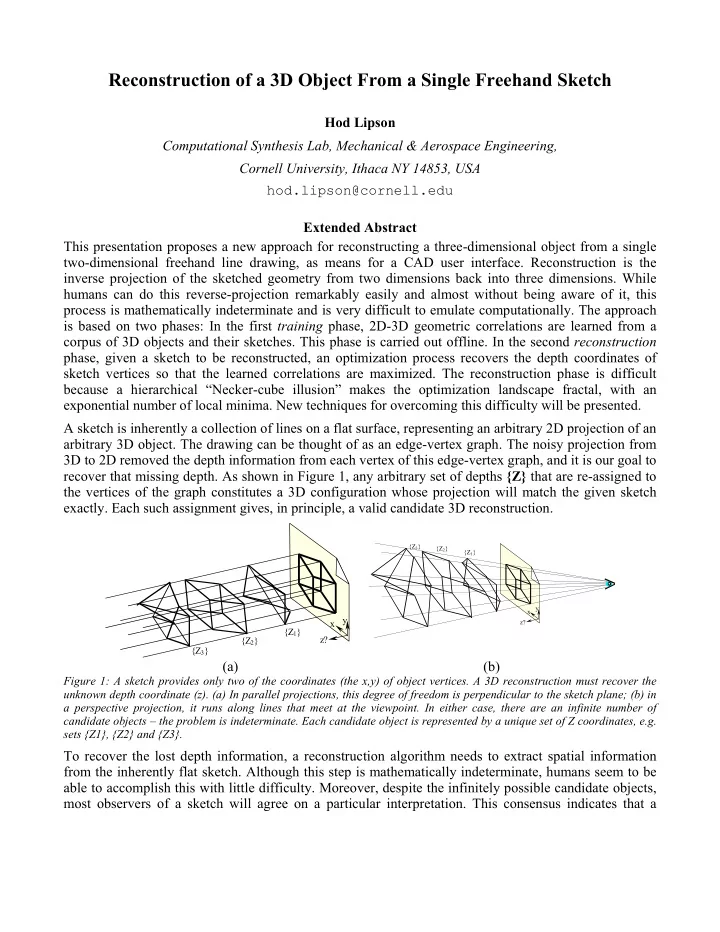
Hod Lipson Computational Synthesis Lab, Mechanical & Aerospace Engineering, Cornell University, Ithaca NY 14853, USA hod.lipson@cornell.edu Extended Abstract This presentation proposes a new approach for reconstructing a three-dimensional object from a single two-dimensional freehand line drawing, as means for a CAD user interface. Reconstruction is the inverse projection of the sketched geometry from two dimensions back into three dimensions. While humans can do this reverse-projection remarkably easily and almost without being aware of it, this process is mathematically indeterminate and is very difficult to emulate computationally. The approach is based on two phases: In the first training phase, 2D-3D geometric correlations are learned from a corpus of 3D objects and their sketches. This phase is carried out offline. In the second reconstruction phase, given a sketch to be reconstructed, an optimization process recovers the depth coordinates of sketch vertices so that the learned correlations are maximized. The reconstruction phase is difficult because a hierarchical “Necker-cube illusion” makes the optimization landscape fractal, with an exponential number of local minima. New techniques for overcoming this difficulty will be presented. A sketch is inherently a collection of lines on a flat surface, representing an arbitrary 2D projection of an arbitrary 3D object. The drawing can be thought of as an edge-vertex graph. The noisy projection from 3D to 2D removed the depth information from each vertex of this edge-vertex graph, and it is our goal to recover that missing depth. As shown in Figure 1, any arbitrary set of depths {Z} that are re-assigned to the vertices of the graph constitutes a 3D configuration whose projection will match the given sketch

• exactly. Each such assignment gives, in principle, a valid candidate 3D reconstruction.

x y z? {Z1} {Z3} {Z2}

x y z? {Z1} {Z3} {Z2}

(a) (b)

Figure 1: A sketch provides only two of the coordinates (the x,y) of object vertices. A 3D reconstruction must recover the unknown depth coordinate (z). (a) In parallel projections, this degree of freedom is perpendicular to the sketch plane; (b) in a perspective projection, it runs along lines that meet at the viewpoint. In either case, there are an infinite number of candidate objects – the problem is indeterminate. Each candidate object is represented by a unique set of Z coordinates, e.g. sets {Z1}, {Z2} and {Z3}.

To recover the lost depth information, a reconstruction algorithm needs to extract spatial information from the inherently flat sketch. Although this step is mathematically indeterminate, humans seem to be able to accomplish this with little difficulty. Moreover, despite the infinitely possible candidate objects, most observers of a sketch will agree on a particular interpretation. This consensus indicates that a

sketch may contain additional information that makes observers agree on the most plausible

• interpretation. A number of approaches have been proposed [5]. These are not surveyed in this abstract.

The proposed approach comprises three phases: (a) The learning phase, where a computer learns the statistical correlations between 3D objects, projections, drawing styles, and 2D drawings, and encodes these correlations in a compact form like a neural network, a Bayesian network, or a probability density

• function. This stage is done offline using a large corpus of training sketches and models. (b) The

inflation phase – for a given sketch, an optimization processes tries to find the optimal depth of the vertices of the sketch such that it matches the previously learned correlations. (c) The fleshing phase – wraps surfaces around the wireframe and transforms it to a solid model. This presentation focuses on the first two stages. We define a 3D-2D geometric correlation as the probability that a certain 2D configuration represents a certain 3D configuration. For example, consider Figure 2a below. The 3D line-pair AB creates a 3D angle α3D=∠AB. When the line pair is projected onto the sketch plane, it produces line-pair ab. The projected angle is α2D=∠ab. Measuring correlation between α3D and α2D over many arbitrary projections of objects in a certain repertoire, we can derive the probability density function pdf(α3D, α2D) for that repertoire of objects and projections. We can then use this probability density function (PDF) to define a cost function that identifies the most likely 3D object.

A B a b A B a b C c

(a) (b)

Figure 2: Measuring 2D-3D correlations. (a) second order, (b) third order.

Instead of simply measuring angles, we also can measure line lengths. Here we would measure the correlation between length ratio in 3D ρ3D=A/B to length ration in 2D ρ2D=a/b. Similarly, we might chose to correlate A/B with ∠ab, or ∠AB with a/b, and so forth. Moreover, we can expand these correlations to third order, by correlating various length-angle relationships among three lines, such as the cone angle of three lines in 3D A×B⋅C versus the cone angle in 2D min(a⋅b, b⋅c, c⋅a), as shown in Figure 2b. Higher order correlations may also be recorded in the form of trivariate probability density functions (PDFs) such as pdf(α3D, α2D, ρ2D). Increasing the order of the correlations is equivalent to increasing the context-dependency of the reconstruction. A bivariate PDF looks at two drawing segments, whereas trivariate looks at combinations of a larger number of segments. As the order of the learned PDFs is increased, more training data and more efficient PDF learning mechanisms are necessary (e.g. neural or Bayesian networks, instead of a simple lookup table). It is also plausible, based

• n neurological observations of the human visual system, that high-order correlations are combined

hierarchically [7]. The PDFs are essentially convolutions of priors of distributions of geometrical properties of possible

• bjects with geometrical properties of projections. For an ideal case (unbiased object geometry and pure

projections) some relationships can be calculated analytically [4,3], but in practice, depicted objects are drawn from a biased repertoire (they are not uniformly random), projections are noisy, and sketching

styles vary. Figure 3 below shows some 2D PDFs collected for 100,000 randomly generated wedge- intersection scenes with noisy orthographic projections.

0° 2D Angle 180° 18 0° 3D Angle 0° 0.0 2D Length Ratio 1.0 1.0 3D Length Ratio 0.0 0° 2D Angle 180° 1.0 3D Length Ratio 0.0 0.0 2D Cone Span 1.0 1.0 3D Cone Span 0.0

Figure 3: Measuring 2D-3D second order correlations. Dark areas show high correlation. Strips on right and bottom of each table show marginal probabilities. The observed patterns represent heuristics, e.g. the dark corner in the third plot

h

• ing 2D angle α2D in the sketch, and using

pdf(α3D, α2D) to estim

corresponds to an abundance of parallel equal-length lines in wedges.

Once geometric correlation functions are known, it is possible to compute the probability of a particular depth set {Z} being the source of a given 2D sketch. This amounts to measuring a 3D angle α3D of line pairs in the candidate reconstruction, and t e corresp nd ate the probability of α3D given α2D:

) , ( ) , ( ) / (

3 2 3 2 3 2 3 2 3 d d d d d d d d d

pdf pdf p δα α α δα δα α α α α ⋅ = ⋅ ⋅ = ) ( ) (

2 2 2 d d d

pdf pdf α δα α ⋅

where δα’s are uncertainties of the measurements and the sketching process. This probability is accumulated (multiplied) for all line pairs/triplets in the candi (1) date object and the sketch using all learned e number of vertices in the sketch minus one) makes this a difficult combinatorial optimization process.

• nential number of local minima, similar to the

shuffled hierarchical if-and-only-if (HIFF) problem [6]. correlation PDFs, to yield the overall candidate probability. Once the likelihood of a candidate reconstruction can be calculated as above, then the reconstruction process ‘amounts’ to an optimization problem, where the objective is to find a set of depth coordinates {Z} that maximizes the likelihood. The high dimensionality of the search space (equal to th We now understand properties of this optimization landscape that suggest why the 2D to 3D reconstruction process does not scale well with standard optimization techniques: It has a fractal

• substructure. For any given solution set Z, the inverse solution –Z is also equally valid (this is known as

the Necker cube illusion). However, this is true not only for the entire drawing, but also for parts of it: For example, there are two equivalent global optima for interpreting a drawing of a block – the forward and the reverse solutions. The next closest sub-optima will be a block with one side interpreted with the forward solution, and the other side with the reverse solution – but that solution is furthest away from the optimal solutions in the search space (Hamming distance). This structure continues recursively, so that the search space has a fractal structure with an exp We have recently developed new large-scale optimization methods suitable for this type of problem [8]. Our method, based on identifying coupling between degrees of freedom and decomposing the problem, has been shown to significantly outperform standard large-scale optimizers, such as simulated annealing and genetic algorithms, for problems with a high degree of coupling such as the sketch reconstruction

• problem. The method uses the eigenvectors of the Hessian of the cost function to dynamically transform

the problem space so that linkage is tight: Linkage is the relationship between the functional dependency among parameters and their proximity in the problem representation. It is a key to the success of a decomposition-based optimizer like an evolutionary algorithm. A performance comparison using our

• ptim

ation andscapes

1000 2000 3000 4000 5000 8 10 12

izer compared to a standard optim [1] is shown in Figure 4.

14 16 18 20 22 24 26 28 30 32 34 36 38 40 42 44 46 48

izer on a real-valued vari

• f Kaufmann’s NK-l

Parallel Hillclimber GA (Standard, with Diversity) GA (Eigenvectors, with Diversity)

Best Fitness

1 2 3 4 5

N=64 N=32 N=16

Factor of Improvement

Figure 4. Performance of new optimization algorithm [8]: (a) on a shuffled real- valued nk landscape [1] w n=64 and k=8. (b) Fac

Generations

(a)

0.0 0.2 0.4 .6 0.8 1.0

Coupling (K / N)

(b

ith tor of improvement on a range of large coupled problems. Statistics for 10 runs.

sketch input without any intermediate human intervention, and during its ) Preliminary results We tested the proposed principles on a few simple line drawings [2], using a simple lookup-table for 2D PDFs and a simple gradient optimizer. The results are displayed as an input line drawing, and the resulting 3D solution rendered from multiple viewpoints with arbitrarily colored faces. The output was generated automatically directly from the without specification of heuristics. Figure 5 shows two structures, not seen by the system training period, reconstructed correctly.

• 2. Li

single freehand sketch", AAAI

• 3. P

ncertainty”, Proceedings

• 4. U

aints for interpretation of line drawings under perspective projections”, Computer

• 5. W

2 pp. 137-158 ). Angeline, Michalewicz, Schoenauer, Yao, Zalzala, eds. IEEE

• 7. W

rarchy of Processing Memories in the Human Visual System”, The American Physical Society, 17-21 March 1997, Kansas City, MO

• 8. Wyatt D, Lipson H., (2003) “Finding Building Blocks Through Eigenstructure Adaptation”, Genetic and Evolutionary

Computation Conference (GECCO ’03) Figure 5: 2D Single freehand sketch input (left) and views of automatically generated 3D reconstruction.

References

• 1. Kauffman, S., (1993) The Origins of Order: Self-Organization and Selection in Evolution. Oxford University Pres.

pson H., Shpitalni M., 2002, "Correlation-based reconstruction of a 3D object from a Spring Symposium on Sketch Understanding, pp. 99-104

• nce J., Shimshoni I., 1992, “An algebraic approach to line drawing analysis in the presence of u
• f the 1992 IEEE Int. Conf. On Robotics and Automation, Nice, France, pp. 1786-1791

lupinar F., Nevatia R., 1991, “Constr Vision Graphics Image Processing (CVGIP): Image Understanding, Vol. 53, No. 1, pp. 88-96. ang W., Grinstein G., 1993, “A survey of 3D solid reconstruction from 2D projection line drawings” Computer Graphics forum Vol. 1

• 6. Watson, R.A. and Pollack, J.B. (1999). Hierarchically-Consistent Test Problems for Genetic Algorithms, Proceedings of

1999 Congress on Evolutionary Computation (CEC 99 Press, pp.1406-1413 illiamson SJ, Uusitalo MA (1997) “Hie