f x , y is F u ,v = i2 xu yv dx dy f - PDF document

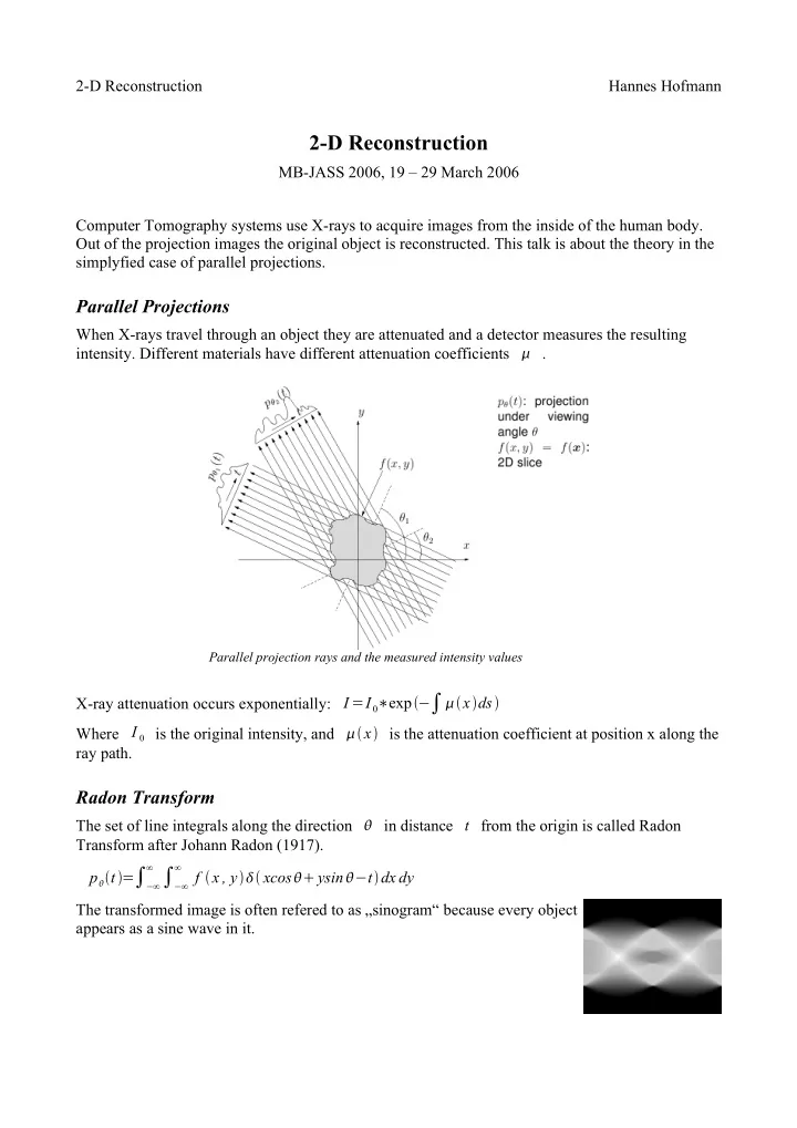
2-D Reconstruction Hannes Hofmann 2-D Reconstruction MB-JASS 2006, 19 – 29 March 2006 Computer Tomography systems use X-rays to acquire images from the inside of the human body. Out of the projection images the original object is reconstructed. This talk is about the theory in the simplyfied case of parallel projections. Parallel Projections When X-rays travel through an object they are attenuated and a detector measures the resulting intensity. Different materials have different attenuation coefficients  . Parallel projection rays and the measured intensity values X-ray attenuation occurs exponentially: I = I 0 ∗ exp − ∫  x  ds  Where I 0 is the original intensity, and  x  is the attenuation coefficient at position x along the ray path. Radon Transform The set of line integrals along the direction  in distance t from the origin is called Radon Transform after Johann Radon (1917). ∞ ∫ −∞ ∞ p   t = ∫ −∞ f  x , y  xcos  ysin − t  dx dy The transformed image is often refered to as „sinogram“ because every object appears as a sine wave in it.

2-D Reconstruction Hannes Hofmann Fourier Slice Theorem f  x , y  in y-direction is defined by the integral The projection of the object ∞ p = 0  x = ∫ f  x , y  dy −∞ ∞ ∫ ∞ f  x , y  is F  u ,v = ∫ −∞ − i2  xu  yv  dx dy f  x , y  e Moreover the Fourier transform of −∞ A slice s  u  through the transformed in angle = 0 is ∞ ∫ −∞ ∞ s  u = F  u ,0 = ∫ − i2  xu dx dy f  x , y  e −∞ ∞ ∞ = ∫ [ ∫ − i2  xu dx f  x , y  dy ] e −∞ −∞ ∞ − i2  tu dt = ∫ p = 0  t  e −∞ p = 0  x  which in turn is the Fourier transform of the projection (A formal derivation for arbitrary angles can be found e.g. in Kak & Slaney) t p   t  P   w  f  x , y  F  u ,v    That means that it would be possible to perfectly reconstruct any object if we had an infinite number of projections. Just find the inverse Radon transform and apply it. Unfortunately the data of that patient would be of no use as he would be dead.

2-D Reconstruction Hannes Hofmann FST – Regridding t P   w  p   t  F  u ,v  f  x , y   In practice we have only a limited number of projections. The projection data lies on circles (dots in the right half) and has to be interpolated into a Carthesian coordinate system. For higher frequency regions (i.e. regions with more details) the sampling density decreases and thus the interpolation result gets worse. Unfiltered Backprojection As expected the reconstruction using the original projection data results in an unsharp and blurred image. Unfiltered backprojection using 180 projections

2-D Reconstruction Hannes Hofmann Filtering The ideal is approximated by a Ideal case Fourier Slice Theorem weightening (highpass) The common approach to counteract the consequenses of the Fourier Slice Theorem is to apply a weighting to the projection data. Filtered Backprojection The interpolation step required by regridding can be avoided if we switch the coordinate system in the frequency domain to the polar coordinate system. Therefore in the formula for the inverse Fourier transform f  x , y = ∫ ∞ ∫ i2  ux  vy  dudv ∞ F  u ,v  e −∞ −∞ we have to substitude u = wcos  v = wsin  and du dv = w dwd  2  ∫ 0 ∞ f  x , y = ∫ 0 i2  xcos  ysin  w dwd  F  w ,  e This can be split into two  ∫ 0 ∞ f  x , y = ∫ 0 i2  xcos  ysin  wdwd  F  w ,  e  ∫ 0 ∞  ∫ 0 i2  xcos  ysin  wdw d  F  w ,  e and with the 180° symmetry of the Fourier transformed F  u , = F − u ,  the equation can be expressed as  ∞ i2  wt dw ] d  f  x , y = ∫ 0 [ ∫ F  w , ∣ w ∣ e −∞ where t is t = xcos  ysin 

2-D Reconstruction Hannes Hofmann We now make use of the FST by substituting the Fourier transform of the projection for the two- dimensional Fourier transform  ∞ i2  wt dw ] d  f  x , y = ∫ 0 [ ∫ −∞ P   w ∣ w ∣ e Which may be written as  f  x , y = ∫ 0 Q   t  d  i2  wt dw ∞ Q   t = ∫ P   w ∣ w ∣ e −∞ Q is the filtered projection with filter function ∣ w ∣ Ramp Filter A highpass filter emphasizes the high frequencies so they contribute more to the reconstruction result. Unfortunately the ramp filter also emphasizes noise, so other filters are more common today. For example the Shepp-Logan kernel which puts a little lower emphasis on very high frequencies. Results: Filtered Backprojection Filtered backprojection using 180 projections

2-D Reconstruction Hannes Hofmann Different kernels The opportunity to choose different filters gives doctors the choice to use the one that fits best for what they want to see. A soft kernel gives images with less noise and smoother On the other side images get a higher resolution and areas, but in turn lower resolution. more noise with a sharp kernel. References A. C. Kak and Malcolm Slaney, Principles of Computerized Tomographic Imaging. Society of Industrial and Applied Mathematics, 2001 S. Horbelt, M. Liebling, M. Unser: Filter design for filtered back-projection guided by the interpolation model, Proceedings of the SPIE International Symposium on Medical Imaging: Image Processing (MI'02), San Diego CA, USA, February 24-28, 2002, vol. 4684, Part II, pp. 806-813. http://en.wikipedia.org/wiki/Radon_transform http://en.wikipedia.org/wiki/Projection-slice_theorem J. Hornegger, D. Paulus: Slides to Medical Image Processing B. Heismann: Slides to Medical Imaging http://homepages.inf.ed.ac.uk/rbf/CVonline/LOCAL_COPIES/AV0405/HAYDEN/Slice_Reconstru ction.html http://www.mssl.ucl.ac.uk/www_solar/moses/moses-web/Pages/fourier-slice-theorem.jpg http://www.eng.warwick.ac.uk/~espbc/courses/undergrad/lec13/filtered_backprojection.htm