Time Evolution Time-evolution problems are widely solved in - - PowerPoint PPT Presentation

SLIDE 1

Parareal Acceleration of Matrix Multiplication

Toshiya Takami and Akira Nishida Kyushu University, Japan

• Aug. 30 - Sep. 2, 2011 ParCo2011, Ghent, Belgium

1

Contents

Introduction: Time-domain Decomposition What is Parareal? Parareal-in-Time Algorithm as a Perturbation Application: Series by Matrix-Vector Multiplications Convergence Property Speed-up Ratio and Efficiency Discussion: Applicability to Other Linear Calculations Conclusion

2

Time Evolution

Time-evolution problems are widely solved in scientific simulations described by discretized differential equations. Parallel technique is usually applied through domain decomposition in the space direction, where quantity

• n the surface of each domain must be shared with its

neighbors. On the other hand, efficient parallelism by the time- domain decomposition seems difficult because of its severe dependency on the previous state.

3

Time-domain Parallelism

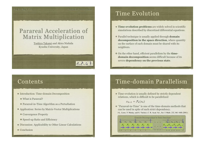
Time-evolution is usually defined by strictly dependent relations, which is difficult to be parallelized ‘’Parareal-in-Time’’ is one of the time-domain methods that can be used in spite of such strict dependency.

x0

t = 0

・・・

1

2

x1 x2 x3

3

F1 F2

・・・ ・・・

xk−1 xk

k − 1 k

Fk−2 F0 Fk−1 F3 Fk−3 Fk−4 F4 F5

4 5 k − 2 k − 3

xk−3 xk−2 x4 x5

Domain Decomposition in Time Direction

xk+1 = Fk(xk)

J-L. Lions, Y. Maday, and G. Turinici, C. R. Acad. Sci., Ser. I: Math. 232, 661–668 (2001).

4

SLIDE 2

What is “Parareal”?

“Its main goal concerns real time problems, hence the proposed terminology of ‘parareal’ algorithm. “Parareal is not the first algorithm to propose the solution of evolution problems in a time-parallel fashion” Multiple Shooting Methods with Newton’s Iterations Space-Time Multigrid Method

• M. J. Gander and S. Vandewalle, SIAM J. Sci. Comput. 29, 556-578 (2007).

J-L. Lions, Y. Maday, and G. Turinici, C. R. Acad. Sci., Ser. I: Math. 232, 661–668 (2001).

5

Parareal-in-Time for Scientific Applications

Since the first proposal by J-L. Lion, et al., various time- evolution problems has been analyzed. PDE with a fluid-structure coupling: Molecular Dynamics with Quantum Iteraction: Quantum Control Problem: Symplectic Integrator:

• L. Baffico, S. Bernard, Y. Maday, G. Turinici, and G. Zérah,
• Phys. Rev. E66, 057701 (2002).
• G. Bal and Q. Wu, LNCSE 60, 401–408 (Springer, 2008).
• C. Farhat and M. Chandesris, Int. J. Numer. Meth. Engng. 58, 1397-1434 (2003).
• Y. Maday, G. Turinici, Int. J. Quant. Chem. 93, 223-228 (2003).

6

Sequence Defined by Parareal-in-Time

Instead of the sequence defined by , consider an approximated one by an iterative relation, where is a coarse evolution that approximates the

• riginal one , and r is the order of the approximation.

The exact operators can be calculated in parallel. In the limit , it has been shown that the approximate sequence converges to the original one: which is called the Parareal-in-Time method. {xk} {x(r)

k }

x(r+1)

k+1

= Gk(x(r+1)

k

) + Fk(x(r)

k ) − Gk(x(r) k )

Gk(·)

Fk(·) r → ∞

{x(r)

k } → {xk}

xk+1 = Fk(xk)

J-L. Lions, Y. Maday, and G. Turinici, C. R. Acad. Sci., Ser. I: Math. 232, 661–668 (2001).

Fk(·)

7

Parareal-in-Time as a Perturbation (1)

While convergence of the Parareal-in-Time method is already shown as the multiple-shooting method, a simple explanation is given here using a linear problem defined by bounded operators: consider a sequence of vectors defined by where we assume and are bounded. Convergence of the sequence above can be explained as a perturbation expansion and the spectral radius of operators.

{xk}

xk+1 = Fkxk = [Gk + (Fk − Gk)] xk

Gk Fk − Gk

8

SLIDE 3

Parareal-in-Time as a Perturbation (2)

For linear problems, the operator is separated into a coarse operator and its correction , If we introduce as r-th order approximation of Thus, the Parareal-in-Time calculations for linear problems can be analyzed as a higher order perturbation.

xk = [Gk−1 + (Fk−1 − Gk−1)] xk−1 =

k−1

• j=0

[Gj + (Fj − Gj)] x0

Fj Gj Fj − Gj x(r+1)

k+1

= [Gk + (Fk − Gk)] x(r+1)

k

= Gkx(r+1)

k

+ (Fk − Gk)x(r+1)

k

≈ Gkx(r+1)

k

+ (Fk − Gk)x(r)

k

{x(r)

k }

{xk}

9

How to Calculate the Parareal Sequence

The parallel procedure of this calculation is: are parallel in k, but are sequantial. k-direction is first, r-direction is sequential

x0 x1 x2 x3 xk−2 xk−1 xk

r = 1 r = 2 r = 3 G F − G

x(3)

k G F − G G F − G G F − G G F − G G F − G

xk−3

F − G G F − G G F − G G F − G G F − G F − G G G G G G r = 0

x(2)

k−1

x(1)

k−2

... ... ... ... ...

G F − G G F − G G F − G G

x4

Order of Perturbation Time

Gk Fk − Gk

10

Series defined by Matrix- Vector Multiplication

A linear time-evolution defined by matrix multiplications, can be represented as an expanded sum in the order of . The third order approximation:

ε

x(3)

k

=

• Gk + ε
• (Terms with a F)

+ε2 (Terms with two F’s) +ε3 (Terms with three F’s)

• x0

xk = (G + εF)xk−1 = (G + εF)kx0

11

Residual Errors from Spectral Radius

Errors can be estimated from the rest of expanded terms: Error from the exact sequence is bounded by By the Stirling’s formula, the magnitude of r-th term is

k

• j=r+1

εj (Terms with F j)x0

• x(r)

k

− x0

• ρ(Gk) |x0| ≤

k

• j=r+1
• k

j ερ(F) ρ(G) j

• k

r ερ(F) ρ(G) r =

• k

2π(k − r)r ek r r ερ(F) ρ(G) r

12

SLIDE 4

Example 1: Real-Symmetric Matrix

Consider a sequence of the real vector defined by a real- symmetrix matrix , where G is diagonal and F is a random matrix with elements satisfying N=1024, =0.01 and in this case, we can set dashed: error of (r+1)-th term

(a) Normalized Error Length of Sequence

• 19
• 17
• 15
• 13
• 11
• 9
• 7
• 5

10 10 10 10 10 10 10 10 r=5 r=10 r=15 50 100 150 200

{xk} G + εF

|Fii|2 = 1 2N , |Fij|2 = 1 4N

ρ(F) ≈ ρ(G) ≈ 1

• 1 1

eigenvalues

• f F

13

Example 2: Unitary Matrix

Unitary time-evolution is often used in quantum mechanics: where H is a Hermitian matrix satisfying N=1024, =0.01 and in this case, we can set dashed: error of (r+1)-th term

(b) Normalized Error Length of Sequence

• 13
• 12
• 11
• 10
• 9
• 8
• 7
• 6
• 5

r=10 r=20 r=30 r=40 r=50 10 10 10 10 10 10 10 10 10 200 400 600 800 1000

xk = exp ∆t i H

• xk−1 ≈ (I − iεH)k x0
• 1 1

eigenvalues

• f H

|Hii|2 = |Hij|2 = 1 4N

ρ(H) ≈ 1

14

Implementation by MPI

We can implement the Parareal-in-Time iteration on parallel computers by the use of MPI_Send/Recv. The original number of calculations, , is compared with the parareal one, .

G G G G G G G G G G G G G G G

F

G

Process 1: Process 2: Process 3: Process 4: Iterate r times P resources KTg + Tc(P − 1) rK(Tf + Tg)/P

F F F F F F F F F F F

Computational Time

K(Tg + Tf) KTg + Tc(P − 1) + rK(Tg + Tf)/P

• E. Aubanel, Parallel Computing 37, 172-182 (2011).

15

Estimation of Speed-up Ratio

Speed-up Ratio will be represented in the function, where and . Property of the Speed-up:

• Max. Efficiency: small P
• Max. Speed-up:

Speedup Ratio Total Number of Ranks (P)

Limit of Speedup K>>P>>1 K~P

• Max. Efficiency (1/r)

1/T K

S(r, K, P) = K(Tg + Tf) KTg + Tc(P − 1) + rK(Tf + Tg) P = P r + TP + P(P − 1) K t

T ≡ Tg/(Tg + Tf) t ≡ Tc/(Tg + Tf)

K ≫ P ≫ 1

16

SLIDE 5

Parallel Performance

• n a Cluster Machine

The performance of the Parareal method is studied on a cluster with 768 cores (Westmere 12 cores x 64 nodes). When we increase the order r of the parareal iterations. Large matrix: almost linear Small matrix: not linear (512 parallel execution)

(a) Time (sec) Parareal Iterations

Normal Method Normal Method Parareal (N=1024) Parareal (N=8192) 1 2 5 10 20 50 100 200 500 1000 10 20 30 40 50 17

Speed-up Ratio

The dashed line represents Actual speed-up is almost half of the value by S(r,K,P). Efficiency is very low, which is bounded by 1/r. N=8192: linear speed-up N=1024: saturated

(b) Speedup Ratio Total Number of Rank

L i n e a r S p e e d u p r=10 r=20 r=40 N=8192 N=1024

0.2 0.5 1 2 5 10 20 50 100 1 10 100 1000

S(r, K, P) = P r + TP + P(P − 1) K t

情報処理学会研究報告

図 法と通常計算の速度比較 次計算を 並列で実行した場合の経過時間， 並列 計算でのスピードアップ比．黒のマークは小規模行列の問題 ，白のマークは比較的大規模な行 列の問題 を表す．四角，丸，三角は，それぞれ， 次の計算に対応する． 表 並列計算によるスピードアップ比 P 16 32 64 128 256 512 768 N = 1024 r = 10 0.71 0.88 1.27 1.61 1.62 1.86 1.73 r = 20 0.36 0.61 0.84 1.16 1.38 1.55 1.49 r = 40 0.19 0.35 0.56 0.80 0.89 1.25 1.31 N = 8192 r = 10 0.69 1.35 2.70 5.41 10.68 21.38 30.97 r = 20 0.36 0.71 1.42 2.83 5.56 11.20 16.63 r = 40 0.19 0.37 0.73 1.44 2.80 5.82 8.52

計算時間の比 は， と の計算量を比べることで見積もることは可能だが，実際の 実行時間は他の様々な要因から予測が難しい場合もある．この手法が有効か，そうでないか を決定するには，データ量などに応じた現実の計算性能を正しく考慮する必要がある． 並列計算でのスピードアップ比 行列演算を 法で並列化した場合の経過時間を， を持つ並列クラスタで測定した．結果を図 に示すが，ここでは，量子力学の 時間発展をモデル化したユニタリ行列 第 節 を対象とし，長さが の複素ベクト ル列 の計算に対して測定した．図 では， 並列実行時の計算時間を， 法の次数に対してプロットした．水平の線は，並列化していない従来法で の時間を表す． の場合，次数 から に対して， 秒から 秒の計 算時間になっており，図ではわかりにくいが にほぼ線形の関係にある．また， で

図

の従来法での計算が 秒であるので，スピードアップは 倍から 倍である．一 方，小さい行列 に対して，スピードアップ比は 程度と小さくなっている． 図 には，次数 に対するスピードアップ比を示す．フラット に よる分散並列化で， プロセスから プロセスまでの結果である． の場合に， と通信の時間を無視した時の，式 の値を図中に点線で示すが，実測値との乖離が 大きい．また，表 に，これらのデータに対応するスピードアップ比の数値を示しておく． スピードアップ比は並列ランク数に比べて低いが， の場合はリニアに伸びてい ることがわかる．つまり，特定の次数の 法は，一定以上大きい行列の計算 に対してはかなり高効率で並列実行できることがわかる．しかし， の場合にはリ ニアな伸びは見られない．これは，式 中の に相当する通信時間の割合が， の時は無視できない事によると思われる． 法の適用範囲 上記の測定と解析の結果， 法が効率的に適用できる行列のサイズと時 系列の長さについて，大まかに図 に示すような分類が出来る．通常の線形ライブラリで は，行列の各要素に対する演算の独立性を利用して，複数のスレッド，あるいは，複数のプ ロセスで並列化されている．行列の対角化が 程度の演算であることより，小さな行 列演算で定義された非常に長い時系列を対象とする場合は，固有状態表現を通して解かれる べきである．大きな行列に対しては の計算量は大きすぎるため， 法による時間方向並列化は，通常の要素方向の並列化法と合わせて解かれるべきである．

18

Applicability to General Iterative Methods

What types of problems can be accelerated by the Parareal? Since the usual row/column parallelism is effectively used in linear libraries, this algorithm should be applied to Long Time Series Large Matrices How about other algorithm?

K ≫ P ≫ 1

cost(G) cost(F)

19

Parareal SOR (preliminary result 1)

In order to solve a linear equation , the SOR (successive over-relaxation) method is used: The parareal accelerated versions are Model 1: is defined as an identity operator: Model 2: is defined by = 0 :

[D + ε(L + U)]x = b xk+1 = (1 − w)xk + w(D + εU)−1[b − εLxk] x(r+1)

k+1

= x(r+1)

k

+ w

• (D + εU)−1[b − εLx(r)

k ] − x(r) k

• G

G

x(r+1)

k+1

= (1 − w)x(r+1)

k

+ wD−1b +w

• (D + εU)−1[b − εLx(r)

k ] − D−1b

• = (1 − w)x(r+1)

k

+ w(D + εU)−1[b − εLx(r)

k ]

20

SLIDE 6

Parareal SOR (preliminary result 2)

The parareal converges to the exact sequence only for w<1, while w is usually chosen 1<w<2 (graphs below: w=0.2). Applicable only for the case of slow convergence?

Difference Iterations

• 8
• 7
• 6
• 5
• 4
• 3
• 2
• 1

10 10 10 10 10 10 10 10 10 r=10 r=20 r=30 r=40 r=50 20 40 60 80 100

Model 1 Model 2

Difference Iterations

• 8
• 7
• 6
• 5
• 4
• 3
• 2
• 1

10 10 10 10 10 10 10 10 10 r=10 r=20 r=30 r=40 50 100 150 200 21

Conclusion

The Parareal-in-Time method for linear evolution problems was analyzed as a perturbation expansion. Remaining errors were obtained through spectral radius

• f the coarse and fine transformation.

A simple linear transformation (matrix multiplication) was accelerated by the Parareal-in-Time algorithm. Convergence properties were analyzed. The speed-ups were compared to the theoretical estimate.

22

Further Studies

How to include this algorithm into parallel linear libraries. interfaces, implementations, tuning, ... hybrid parallel implementations with the parareal-in-time and the usual row/column parallelisms How wide is this algorithm applied to linear calculations such as iterative solvers of linear equations: SOR, CG, etc? Application of this method in massively parallel computers such as K-computer, Kobe, Japan.

23

Thank you for your attention.

24