parallel in time integration with pfasst from prototyping
play

Parallel-in-Time Integration with PFASST From prototyping to - PowerPoint PPT Presentation

Parallel-in-Time Integration with PFASST From prototyping to applications June 5, 2019 Robert Speck Jlich Supercomputing Centre Member of the Helmholtz Association Collaborators Daniel Ruprecht Rolf Krause Oliver Sander Matthias Bolten


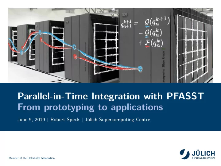
  1. Parallel-in-Time Integration with PFASST From prototyping to applications June 5, 2019 Robert Speck Jülich Supercomputing Centre Member of the Helmholtz Association
  2. Collaborators Daniel Ruprecht Rolf Krause Oliver Sander Matthias Bolten You? Michael Minion Member of the Helmholtz Association June 5, 2019 Slide 1

  3. Moore’s law in HPC today "The free lunch is over” (H.Sutter, 2005) 10 7 10 6 10 5 Cores 10 4 10 3 10 2 1995 2000 2005 2010 2015 2020 Year (a) Performance of the world’s 500 most powerful (b) Number of cores in the number one system in supercomputers. the Top 500 list. HPC systems already require multi-million way concurrency Need new numerical methods to provide this degree of parallelism Member of the Helmholtz Association June 5, 2019 Slide 2

  4. Limits of purely spatial parallelization Time Figure: Time-stepping to solve time-dependent partial differential equations. Spatial parallelization reduces runtime per time-step Strong scaling saturates eventually because of communication Costs for more time-steps are not mitigated Member of the Helmholtz Association June 5, 2019 Slide 3

  5. Limits of purely spatial parallelization Figure: Time-stepping to solve time-dependent partial differential equations. Spatial parallelization reduces runtime per time-step Strong scaling saturates eventually because of communication Costs for more time-steps are not mitigated Member of the Helmholtz Association June 5, 2019 Slide 3

  6. Limits of purely spatial parallelization Time Figure: Time-stepping to solve time-dependent partial differential equations. Spatial parallelization reduces runtime per time-step Strong scaling saturates eventually because of communication Costs for more time-steps are not mitigated Member of the Helmholtz Association June 5, 2019 Slide 3

  7. Limits of purely spatial parallelization Time Figure: Time-stepping to solve time-dependent partial differential equations. Spatial parallelization reduces runtime per time-step Strong scaling saturates eventually because of communication Costs for more time-steps are not mitigated Member of the Helmholtz Association June 5, 2019 Slide 3

  8. Limits of purely spatial parallelization Time Figure: Time-stepping to solve time-dependent partial differential equations. Spatial parallelization reduces runtime per time-step Strong scaling saturates eventually because of communication Costs for more time-steps are not mitigated → Can we compute multiple time-steps simultaneously? Member of the Helmholtz Association June 5, 2019 Slide 3

  9. Parallel-in-Time (“PinT”) approaches “50 years of parallel-in-time integration”, M. Gander ( CMCS, 2015) Interpolation-based approach (Nievergelt 1964) Predictor-corrector approach (Miranker, Liniger 1967) Parabolic or time multi-grid (Hackbusch 1984) and (Horton 1992) Multiple shooting in time (Kiehl 1994) Parallel Runge-Kutta methods (e.g. Butcher 1997) Parareal (Lions, Maday, Turinici 2001) PITA (Farhat, Chandesris 2003) Guided Simulations (Srinavasan, Chandra 2005) RIDC (Christlieb, Macdonald, Ong 2010) PFASST (Emmett, Minion 2012) MGRIT (Falgout et al 2014) ... and many more Member of the Helmholtz Association June 5, 2019 Slide 4

  10. Parallel-in-Time (“PinT”) approaches “50 years of parallel-in-time integration”, M. Gander ( CMCS, 2015) Interpolation-based approach (Nievergelt 1964) Predictor-corrector approach (Miranker, Liniger 1967) Parabolic or time multi-grid (Hackbusch 1984) and (Horton 1992) Multiple shooting in time (Kiehl 1994) Parallel Runge-Kutta methods (e.g. Butcher 1997) Parareal (Lions, Maday, Turinici 2001) PITA (Farhat, Chandesris 2003) Guided Simulations (Srinavasan, Chandra 2005) RIDC (Christlieb, Macdonald, Ong 2010) PFASST (Emmett, Minion 2012) MGRIT (Falgout et al 2014) ... and many more Member of the Helmholtz Association June 5, 2019 Slide 4

  11. <math>

  12. A quick algebraic introduction to PFASST Basic building block: spectral deferred corrections (SDC) Consider the Picard form of an initial value problem on [ T 0 , T 1 ] � t u ( t ) = u 0 + f ( u ( s )) ds , T 0 discretized using spectral quadrature rules with nodes t m : � t m u m = u 0 + ∆ tQF ( u ) ≈ u 0 + f ( u ( s )) ds , T 0 then SDC methods can be seen as (clever) Gauß-Seidel iteration to solve this collocation problem for all u m . ⇒ Use this for block smoothing in space-time multigrid = PFASST Member of the Helmholtz Association June 5, 2019 Slide 5

  13. A quick algebraic introduction to PFASST Basic building block: spectral deferred corrections (SDC) Consider the Picard form of an initial value problem on [ T 0 , T 1 ] � t u ( t ) = u 0 + f ( u ( s )) ds , T 0 discretized using spectral quadrature rules with nodes t m : ( I − ∆ tQF )( � u ) = � u 0 then SDC methods can be seen as (clever) Gauß-Seidel iteration to solve this collocation problem for all u m . ⇒ Use this for block smoothing in space-time multigrid = PFASST Member of the Helmholtz Association June 5, 2019 Slide 5

  14. A quick algebraic introduction to PFASST Multigrid for the composite collocation problem We now glue L time-steps together, using N to transfer information from step l to step l + 1. We get the composite collocation problem:       I − ∆ tQF � � u 1 u 0 − N I − ∆ tQF u 2 � 0        =    .   .  ... ... . .       . .      I − ∆ tQF 0 − N � u L PFASST : use (linear/FAS) multigrid to solve this system iteratively smoother: parallel block Jacobi with SDC in the blocks coarse-level solver: serial block Gauß-Seidel with SDC in the blocks exploit cheapest coarse level to quickly propagate information forward in time Member of the Helmholtz Association June 5, 2019 Slide 6

  15. </math>

  16. A quick visual introduction to PFASST coarse sweep fine computation time sweep coarse comm. fine comm. predictor t 0 t 1 t 2 t 3 t 4 P 0 P 1 P 2 P 3 Member of the Helmholtz Association June 5, 2019 Slide 7

  17. A quick visual introduction to PFASST coarse sweep fine computation time sweep coarse comm. fine comm. predictor t 0 t 1 t 2 t 3 t 4 P 0 P 1 P 2 P 3 Member of the Helmholtz Association June 5, 2019 Slide 7

  18. A quick visual introduction to PFASST coarse sweep fine computation time sweep coarse comm. fine comm. predictor t 0 t 1 t 2 t 3 t 4 P 0 P 1 P 2 P 3 Member of the Helmholtz Association June 5, 2019 Slide 7

  19. A quick visual introduction to PFASST coarse sweep fine computation time sweep coarse comm. fine comm. predictor t 0 t 1 t 2 t 3 t 4 P 0 P 1 P 2 P 3 Member of the Helmholtz Association June 5, 2019 Slide 7

  20. A quick visual introduction to PFASST coarse sweep fine computation time sweep coarse comm. fine comm. predictor t 0 t 1 t 2 t 3 t 4 P 0 P 1 P 2 P 3 Member of the Helmholtz Association June 5, 2019 Slide 7

  21. A quick visual introduction to PFASST coarse sweep fine computation time sweep coarse comm. fine comm. predictor t 0 t 1 t 2 t 3 t 4 P 0 P 1 P 2 P 3 Member of the Helmholtz Association June 5, 2019 Slide 7

  22. A quick visual introduction to PFASST coarse sweep fine computation time sweep coarse comm. fine comm. predictor t 0 t 1 t 2 t 3 t 4 P 0 P 1 P 2 P 3 Member of the Helmholtz Association June 5, 2019 Slide 7

  23. A quick visual introduction to PFASST coarse sweep fine computation time sweep coarse comm. fine comm. predictor t 0 t 1 t 2 t 3 t 4 P 0 P 1 P 2 P 3 Member of the Helmholtz Association June 5, 2019 Slide 7

  24. A quick visual introduction to PFASST coarse sweep fine computation time sweep coarse comm. fine comm. predictor t 0 t 1 t 2 t 3 t 4 P 0 P 1 P 2 P 3 Member of the Helmholtz Association June 5, 2019 Slide 7

  25. A quick visual introduction to PFASST coarse sweep fine computation time sweep coarse comm. fine comm. predictor t 0 t 1 t 2 t 3 t 4 P 0 P 1 P 2 P 3 Member of the Helmholtz Association June 5, 2019 Slide 7

  26. A quick visual introduction to PFASST coarse sweep fine computation time sweep coarse comm. fine comm. predictor t 0 t 1 t 2 t 3 t 4 P 0 P 1 P 2 P 3 Member of the Helmholtz Association June 5, 2019 Slide 7

  27. A quick visual introduction to PFASST coarse sweep fine computation time sweep coarse comm. fine comm. predictor t 0 t 1 t 2 t 3 t 4 P 0 P 1 P 2 P 3 Member of the Helmholtz Association June 5, 2019 Slide 7

  28. A quick visual introduction to PFASST coarse sweep fine computation time sweep coarse comm. fine comm. predictor t 0 t 1 t 2 t 3 t 4 P 0 P 1 P 2 P 3 Member of the Helmholtz Association June 5, 2019 Slide 7

  29. A quick visual introduction to PFASST coarse sweep fine computation time sweep coarse comm. fine comm. predictor t 0 t 1 t 2 t 3 t 4 P 0 P 1 P 2 P 3 Member of the Helmholtz Association June 5, 2019 Slide 7

  30. A quick visual introduction to PFASST coarse sweep fine computation time sweep coarse comm. fine comm. predictor t 0 t 1 t 2 t 3 t 4 P 0 P 1 P 2 P 3 Member of the Helmholtz Association June 5, 2019 Slide 7

  31. A quick visual introduction to PFASST coarse sweep fine computation time sweep coarse comm. fine comm. predictor t 0 t 1 t 2 t 3 t 4 P 0 P 1 P 2 P 3 Member of the Helmholtz Association June 5, 2019 Slide 7

Download Presentation
Download Policy: The content available on the website is offered to you 'AS IS' for your personal information and use only. It cannot be commercialized, licensed, or distributed on other websites without prior consent from the author. To download a presentation, simply click this link. If you encounter any difficulties during the download process, it's possible that the publisher has removed the file from their server.

Recommend


More recommend