Parallel parking a car - PDF document

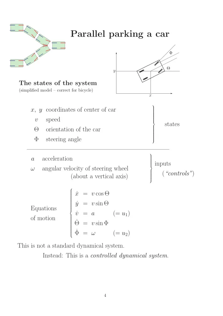
Parallel parking a car � � ✟✟✟✟✟✟ Φ � ✻ � ✟✟✟✟✟✟✟ ✟✟✟✟✟✟ � ❆ � � � ❆ Θ ❆ ✟ ✟ ✟ y ✟ ✟ � ✟ � ✟✟✟✟✟✟ � ❆ ❆ ✟ ✟ ✟ ✟ ✟ ✟ ❆ The states of the system (simplified model – correct for bicycle) ✲ x  x, y coordinates of center of car         speed  v    states Θ orientation of the car          Φ steering angle     acceleration a      inputs    ω angular velocity of steering wheel  ( “controls” )   (about a vertical axis)       x = v cos Θ ˙           y = v sin Θ ˙     Equations    v = a ˙ (= u 1 ) of motion     ˙  Θ = v sin Φ        ˙   Φ = ω (= u 2 )    This is not a standard dynamical system. Instead: This is a controlled dynamical system . 4

Parallel parking a car   x = v cos Θ ˙           y = v sin Θ ˙          v = a ˙ (= u 1 )     ˙  Θ = v sin Φ          ˙  Φ = ω (= u 2 )      Written in standard as a multi-input control system  � 2  z = f 0 ( z ) + ˙ j =1 u j f j ( z )        z ∈ M 5 = R 3 × S 1 × S 1         u ∈ [ − a max , a max ] × [ − ω max , ω max ]     with drift vector field ∂ ∂ ∂ f 0 = z 3 cos z 4 + z 3 sin z 4 + z 3 sin z 5 , ∂z 1 ∂z 2 ∂z 4 and controlled fields f 1 = ∂ f 2 = ∂ , and . ∂z 3 ∂z 5 For every choice of controls u 1 ( t ) , u 2 ( t ) (that are locally integrable) one obtains an ordinary dynamical system. 5

Easiest example: Piecewise constant controls in this simple cascade system Control inputs : Blue: For/backward acceleration u 1 Red: Angular velocity of steering wheel u 2 States : � u 1 Black: For/backward speed v = � u 2 . Magenta: Steering angle Φ = � v sin Φ. Brown: Orientation of the car Θ = Green: x -component of velocity v x = v cos Θ Cyan: y -component of velocity v y = v sin Θ v (0) = Φ(0) = Θ(0) = x (0) = y (0) = 0 = v ( t ) = Φ( t ) = Θ( t ) = x ( t ) Θ( t 1 ) � �� � � t � t 1 � t 1 � t 2 � t 2 y ( t ) = 0 u 1 ( t 2 ) dt 2 · sin ( 0 u 1 ( t 2 ) dt 2 · sin( 0 u 2 ( t 3 ) dt 3 ) dt 2 ) dt 1 0 0 � �� � � �� � � �� � v ( t 1 ) v ( t 2 ) Φ( t 2 ) 6

Noncommuting flows Concatenate the solutions of the (standard) dynamical systems (controls normalized to ± 1) 0 ≤ t < T 1 z = f 0 ( z ) + f 1 ( x ) + f 2 ( z ) ˙ z = f 0 ( z ) + f 1 ( x ) − f 2 ( z ) ˙ T 1 ≤ t < T 2 z = f 0 ( z ) ˙ − f 2 ( z ) T 2 ≤ t < T 3 T 3 ≤ t < T 4 z = f 0 ( z ) − f 1 ( x ) − f 2 ( z ) ˙ T 4 ≤ t < T 5 z = f 0 ( z ) − f 1 ( x ) + f 2 ( z ) ˙ z = f 0 ( z ) − f 1 ( x ) − f 2 ( z ) ˙ T 5 ≤ t < T 6 z = f 0 ( z ) ˙ − f 2 ( z ) T 6 ≤ t < T 7 T 7 ≤ t < T 8 z = f 0 ( z ) + f 1 ( x ) − f 2 ( z ) ˙ z = f 0 ( z ) + f 1 ( x ) + f 2 ( z ) ˙ T 8 ≤ t < T 9 The flows do not commute. 1 z Most simple picture for: 0     1 0 1     0 x     f 1 ( x ) = f 2 ( x ) = 0 1 y     0         1 − y x 7

Parking model is controllable       z 3 cos z 4 0 0             z 3 sin z 4 0 0                         f 0 ( z ) = f 1 ( z ) = f 2 ( z ) = Recall: 0 1 0                         z 3 sin z 5 0 0                   0 0 1       cos z 4 0 0             sin z 4 0 0                         [ f 1 , f 0 ]( x ) = [ f 2 , f 0 ]( x ) = [ f 2 , f 1 ]( x ) = 0 0 0                    sin z 5   z 3 cos z 5   0                    0 0 0     0 sin z 4          0   cos z 4              [ f 1 , [ f 2 , f 0 ]]( x ) = [[ f 1 , [ f 2 , f 0 ]] , [ f 1 , f 2 ]]( x ) = 0 0                 cos z 5 0             0 0 These iterated Lie brackets span the tangent space of R 5 at the origin – hence the system is accessible from 0. 10

Manipulating exponential products Instead of working with complicated concatenations of flows like � t 9 � t 2 � t 1 t 8 ( f 0 + f 1 + f 2 ) dt ◦ . . . e t 1 ( f 0 + f 1 − f 2 ) dt ◦ e 0 ( f 0 + f 1 + f 2 ) dt ( p ) z ( t ) = e it is desirable to rewrite the solution curve using a minimal number of vector fields f π k that span the tangent space (typically using iterated Lie brackets of the system fields f 0 , f 1 , . . . f m ) Coordinates of the first kind z ( t ) = e b 1 ( t,u ) f π 1 + b 2 ( t,u ) f π 1 + b 3 ( t,u ) f π 3 + ... + b n ( t,u ) f πn ( p ) Coordinates of the second kind z ( t ) = e c 1 ( t,u ) f π 1 ◦ e c 2 ( t,u ) f π 1 ◦ e c 3 ( t,u ) f π 3 ◦ . . . ◦ e c n ( t,u ) f πn ( p ) Using the Campbell-Baker-Hausdorff formula , this is possible, but a book-keeping nightmare. Moreover, the CBH formula does not use a basis, but uses linear combinations of all possible iterated Lie brackets. Yet, by the Jacobi identity (and anticommutativity), in ever Lie algebra e.g. [ X, [ Y, [ X, Y ]]] + [ Y, [[ X, Y ] , X ] � ] + [[ X, Y ] , [ X, Y ]]] = 0 � �� and hence � �� � [ X, [ Y, [ X, Y ]]] = [ Y, [ X, [ X, Y ]]] Plan : • Work with bases for (free) Lie algebras. • Find useful formulae for the coefficients b k ( t, u ) or c k ( t, u ). 11

The Chen Fliess series K. T. Chen, 1957: Geometric invariants of curves in R n M. Fliess, 1970s: adaptation to control The formal control system   m ˙ �  , u i X i S = S S (0) = I  i =1 on the associative algebra ˆ A ( X 1 . . . X m ) of formal power series in the noncommuting indeterminates (letters) X 1 , . . . X m has the unique solution � T � t 1 � t p − 1 � u i p ( t p ) . . . u i 1 ( t 1 ) dt 1 . . . dt p S CF ( T, u ) = X i 1 . . . X i p 0 · · · 0 0 I � �� � � �� � X I Υ I ( T,u ) What is the CF-series good for? For any given control system m � x = ˙ u i ( x ) f i ( x ) , x (0) = p, with “output” y = ϕ ( x ) i =1 � T � t 1 � t p − 1 � u i p ( t p ) . . . u i 1 ( t 1 ) dt 1 . . . dt p φ ( x ( T, u )) = ( f i 1 ◦ . . . ◦ f i p ϕ )( p ) 0 · · · 0 0 I � �� � Υ I ( T,u ) (uniform convergence for small T and IC’s on compacta [Sussmann, 1983]) The CF-series was basic tool for deriving many high-order conditions for controllability and optimality. [Hermes, Stefani, Sussmann, Kawski, ...] 12