recap: Overfitting Fitting the data more than is warranted Learning - - PowerPoint PPT Presentation

Learning From Data Lecture 12 Regularization

Constraining the Model Weight Decay Augmented Error

• M. Magdon-Ismail

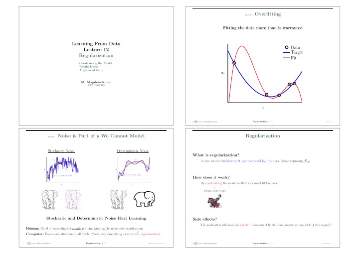
CSCI 4100/6100 recap: Overfitting

Fitting the data more than is warranted

x y Data Target Fit

c A M L Creator: Malik Magdon-Ismail

Regularization: 2 /30

Noise − →

recap: Noise is Part of y We Cannot Model

Stochastic Noise

x y f(x) y = f(x)+stoch. noise

Deterministic Noise

x y h∗ y = h∗(x)+det. noise

Stochastic and Deterministic Noise Hurt Learning

Human: Good at extracting the simple pattern, ignoring the noise and complications. Computer: Pays equal attention to all pixels. Needs help simplifying → (features

• , regularization).

c A M L Creator: Malik Magdon-Ismail

Regularization: 3 /30

What is regularization? − →

Regularization

What is regularization?

A cure for our tendency to fit (get distracted by) the noise, hence improving Eout.

How does it work?

By constraining the model so that we cannot fit the noise. ↑

putting on the brakes

Side effects?

The medication will have side effects – if we cannot fit the noise, maybe we cannot fit f (the signal)?

c A M L Creator: Malik Magdon-Ismail

Regularization: 4 /30

Constraining − →

Constraining the Model: Does it Help?

x y

. . . and the winner is:

c A M L Creator: Malik Magdon-Ismail

Regularization: 5 /30

Small weights − →

Constraining the Model: Does it Help?

x y x y

constrain weights to be smaller

. . . and the winner is:

c A M L Creator: Malik Magdon-Ismail

Regularization: 6 /30

bias− →

Bias Goes Up A Little

x y ¯ g(x) sin(x) x y ¯ g(x) sin(x)

no regularization bias = 0.21 regularization bias = 0.23

← side effect (Constant model had bias=0.5 and var=0.25.)

c A M L Creator: Malik Magdon-Ismail

Regularization: 7 /30

var− →

Variance Drop is Dramatic!

x y ¯ g(x) sin(x) x y ¯ g(x) sin(x)

no regularization bias = 0.21 var = 1.69 regularization bias = 0.23

← side effect

var = 0.33

← treatment (Constant model had bias=0.5 and var=0.25.)

c A M L Creator: Malik Magdon-Ismail

Regularization: 8 /30

Regularication in a nutshell − →

Regularization in a Nutshell

VC analysis: Eout(g) ≤ Ein(g) + Ω(H) տ

If you use a simpler H and get a good fit, then your Eout is better.

Regularization takes this a step further: If you use a ‘simpler’ h and get a good fit, then is your Eout better?

c A M L Creator: Malik Magdon-Ismail

Regularization: 9 /30

Polynomials − →

Polynomials of Order Q - A Useful Testbed

Hq: polynomials of order Q.

Standard Polynomial Legendre Polynomial z =        1 x x2 . . . xq        h(x) = wtz(x) = w0 + w1x + · · · + wqxq z =        1 L1(x) L2(x) . . . Lq(x)        h(x) = wtz(x) = w0 + w1L1(x) + · · · + wqLq(x)

ւ

we’re using linear regression

տ

allows us to treat the weights ‘independently’

L1

x

L2

1 2(3x2 − 1)

L3

1 2(5x3 − 3x)

L4

1 8(35x4 − 30x2 + 3)

L5

1 8(63x5 · · · )

c A M L Creator: Malik Magdon-Ismail

Regularization: 10 /30

recap: linear regression − →

recap: Linear Regression

(x1, y1), . . . , (xN, yN)

• X y

− → (z1, y1), . . . , (zN, yN)

• Z y

min : Ein(w) = 1 N

N

• n=1

(wtzn − yn)2 = 1 N (Zw − y)t(Zw − y) wlin = (ZtZ)−1Zty

linear regression fit ր

c A M L Creator: Malik Magdon-Ismail

Regularization: 11 /30

Already saw constraints − →

Constraining The Model: H10 vs. H2

H10 =

• h(x) = w0 + w1Φ1(x) + w2Φ2(x) + w3Φ3(x) + · · · + w10Φ10(x)
• H2 =

h(x) = w0 + w1Φ1(x) + w2Φ2(x) + w3Φ3(x) + · · · + w10Φ10(x)

such that: w3 = w4 = · · · = w10 = 0

• a ‘hard’ order constraint that

sets some weights to zero ր

H2 ⊂ H10

c A M L Creator: Malik Magdon-Ismail

Regularization: 12 /30

Soft constraint − →

Soft Order Constraint

Don’t set weights explicitly to zero (e.g. w3 = 0). Give a budget and let the learning choose.

q

• q=0

w2

q ≤ C տ

budget for weights H2 C → ∞ H10

soft order constraint allows ‘intermediate’ models c A M L Creator: Malik Magdon-Ismail

Regularization: 13 /30

HC − →

Soft Order Constrained Model HC

H10 =

• h(x) = w0 + w1Φ1(x) + w2Φ2(x) + w3Φ3(x) + · · · + w10Φ10(x)
• H2 =

h(x) = w0 + w1Φ1(x) + w2Φ2(x) + w3Φ3(x) + · · · + w10Φ10(x)

such that: w3 = w4 = · · · = w10 = 0

• HC =

     h(x) = w0 + w1Φ1(x) + w2Φ2(x) + w3Φ3(x) + · · · + w10Φ10(x)

such that:

10

• q=0

w2

q ≤ C

    

a ‘soft’ budget constraint

• n the sum of weights

ր

VC-perspective: HC is smaller than H10 = ⇒ better generalization.

c A M L Creator: Malik Magdon-Ismail

Regularization: 14 /30

Fitting data − →

Fitting the Data

The optimal weights wreg ∈ HC

regularized ր

should minimize the in-sample error, but be within the budget. wreg is a solution to min : Ein(w) = 1 N (Zw − y)t(Zw − y)

subject to:

wtw ≤ C

c A M L Creator: Malik Magdon-Ismail

Regularization: 15 /30

Getting wreg − →

Solving For wreg

min : Ein(w) = 1 N (Zw − y)t(Zw − y)

subject to:

wtw ≤ C Observations:

• 1. Optimal w tries to get as ‘close’ to wlin as possible.

Optimal w will use full budget and be on the surface wtw = C.

• 2. Surface wtw = C, at optimal w, should be perpindicular to ∇Ein.

Otherwise can move along the surface and decrease Ein.

• 3. Normal to surface wtw = C is the vector w.
• 4. Surface is ⊥ ∇Ein; surface is ⊥ normal.

∇Ein is parallel to normal (but in opposite direction).

∇Ein(wreg) = −2λCwreg

wlin wtw = C w Ein = const. ∇Ein normal

λC, the lagrange multiplier, is positive. The 2 is for mathematical convenience.

ր

c A M L Creator: Malik Magdon-Ismail

Regularization: 16 /30

Unconstrained minimization − →

Solving For wreg

Ein(w) is minimized, subject to: wtw ≤ C ⇔ ∇Ein(wreg) + 2λCwreg = 0 ⇔ ∇ (Ein(w) + λCwtw)

• w=wreg = 0

⇔ Ein(w) + λCwtw is minimized, unconditionally There is a correspondence: C ↑ λC ↓

c A M L Creator: Malik Magdon-Ismail

Regularization: 17 /30

Augmented error − →

The Augmented Error

Pick a C and minimize Ein(w) subject to: wtw ≤ C

• Pick a λC and minimize

Eaug(w) = Ein(w) + λCwtw unconditionally

տ

A penalty for the ‘complexity’ of h, measured by the size of the weights.

We can pick any budget C. Translation: we are free to pick any multiplier λC What’s the right C? ↔ What’s the right λC?

c A M L Creator: Malik Magdon-Ismail

Regularization: 18 /30

Linear regression − →

Linear Regression With Soft Order Constraint

Eaug(w) = 1 N (Zw − y)t(Zw − y) + λCwtw տ

Convenient to set λC = λ

N

Eaug(w) = (Zw − y)t(Zw − y) + λwtw N տ

called ‘weight decay’ as the penalty encourages smaller weights

Unconditionally minimize Eaug(w).

c A M L Creator: Malik Magdon-Ismail

Regularization: 19 /30

Linear regression solution − →

The Solution for wreg

∇Eaug(w) = 2Zt(Zw − y) + 2λw = 2(ZtZ + λI)w − 2Zty Set ∇Eaug(w) = 0 wreg = (ZtZ + λI)−1Zty ↑

λ determines the amount of regularization

Recall the unconstrained solution (λ = 0):

wlin = (ZtZ)−1Zty

c A M L Creator: Malik Magdon-Ismail

Regularization: 20 /30

Dramatic effect − →

A Little Regularization . . .

Minimizing Ein(w) + λ N wtw with different λ’s λ = 0 λ = 0.0001

x y Data Target Fit

Overfitting Wow!

c A M L Creator: Malik Magdon-Ismail

Regularization: 21 /30

Just a little works − →

. . . Goes A Long Way

Minimizing Ein(w) + λ N wtw with different λ’s λ = 0 λ = 0.0001

x y Data Target Fit x y

Overfitting Wow!

c A M L Creator: Malik Magdon-Ismail

Regularization: 22 /30

Easy to overdose − →

Don’t Overdose

Minimizing Ein(w) + λ N wtw with different λ’s λ = 0 λ = 0.0001 λ = 0.01 λ = 1

x y Data Target Fit x y x y x y

Overfitting

→ →

Underfitting

c A M L Creator: Malik Magdon-Ismail

Regularization: 23 /30

Overfitting and underfitting − →

Overfitting and Underfitting

Regularization Parameter, λ Expected Eout

• verfitting

underfitting

0.5 1 1.5 2 0.76 0.8 0.84

c A M L Creator: Malik Magdon-Ismail

Regularization: 24 /30

Noise and regularization − →

More Noise Needs More Medicine

Regularization Parameter, λ Expected Eout σ2 = 0 σ2 = 0.25 σ2 = 0.5

0.5 1 1.5 2 0.25 0.5 0.75 1

c A M L Creator: Malik Magdon-Ismail

Regularization: 25 /30

Deterministic too − →

. . . Even For Deterministic Noise

Regularization Parameter, λ Expected Eout σ2 = 0 σ2 = 0.25 σ2 = 0.5

0.5 1 1.5 2 0.25 0.5 0.75 1

Regularization Parameter, λ Expected Eout Qf = 15 Qf = 30 Qf = 100

0.5 1 1.5 2 0.2 0.4 0.6

c A M L Creator: Malik Magdon-Ismail

Regularization: 26 /30

Variations on weight decay − →

Variations on Weight Decay

Uniform Weight Decay Low Order Fit Weight Growth!

Regularization Parameter, λ Expected Eout

• verfitting

underfitting

0.5 1 1.5 2 0.76 0.8 0.84

Regularization Parameter, λ Expected Eout

0.5 1 1.5 2 0.76 0.8 0.84

Regularization Parameter, λ Expected Eout weight growth weight decay

Q

• q=0

w2

q Q

• q=0

qw2

q Q

• q=0

1 w2

q

c A M L Creator: Malik Magdon-Ismail

Regularization: 27 /30

Choosing a regularizer − →

Choosing a Regularizer – A Practitioner’s Guide

The perfect regularizer:

constrain in the ‘direction’ of the target function. target function is unknown (going around in circles ).

The guiding principle:

constrain in the ‘direction’ of smoother (usually simpler) hypotheses hurts your ability to fit the ‘high frequency’ noise smoother and simpler

usually means

− → weight decay not weight growth.

What if you choose the wrong regularizer?

You still have λ to play with — validation.

c A M L Creator: Malik Magdon-Ismail

Regularization: 28 /30

Regularization philosophy − →

How Does Regularization Work?

Stochastic noise − → nothing you can do about that. Good features − → helps to reduce deterministic noise. Regularization:

Helps to combat what noise remains, especially when N is small. Typical modus operandi: sacrifice a little bias for a huge improvement in var. VC angle: you are using a smaller H without sacrificing too much Ein

c A M L Creator: Malik Magdon-Ismail

Regularization: 29 /30

Eaug versus Ein − →

Augmented Error as a Proxy for Eout

Eaug(h) = Ein(h) + λ

NΩ(h)

• Eout(h) ≤ Ein(h) + Ω(H)

ւ

this was wtw

տ

this was O

• dvc

N ln N

• Eaug can beat Ein as a proxy for Eout.

տ

depends on choice of λ

c A M L Creator: Malik Magdon-Ismail

Regularization: 30 /30