cse 446 week 3 decision trees apr 4 instructor sergey
play

CSE 446: Week 3: Decision Trees (Apr 4) Instructor: Sergey Levine - PDF document

CSE 446: Week 3: Decision Trees (Apr 4) Instructor: Sergey Levine I. Overfitting idea 1: holdout crossvalidation What if we could test for overfitting directly while building our tree? Recall what I mentioned about a holdout set in lecture.


  1. CSE 446: Week 3: Decision Trees (Apr 4) Instructor: Sergey Levine I. Overfitting idea 1: holdout cross­validation What if we could test for overfitting directly while building our tree? Recall what I mentioned about a hold­out set in lecture. We can reserve a little piece of data to test for overfitting. It is critical that this piece of data not be used for actually fitting the tree, and it must be distinct from our test (which must be pure and unpolluted and never ever touched during training ever). We 
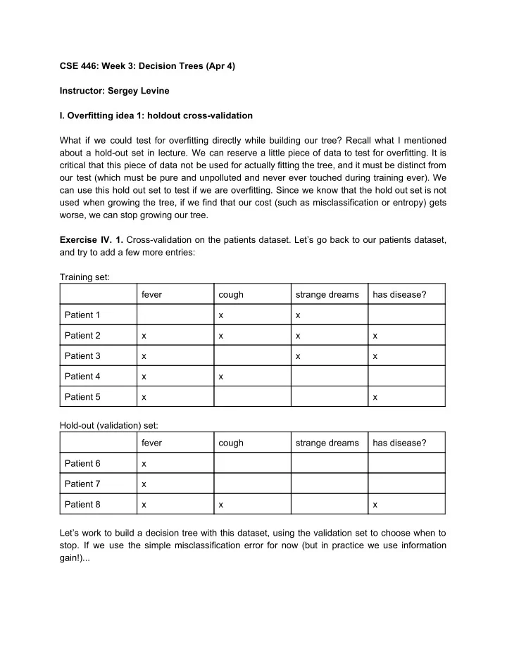
can use this hold out set to test if we are overfitting. Since we know that the hold out set is not used when growing the tree, if we find that our cost (such as misclassification or entropy) gets worse, we can stop growing our tree. Exercise IV. 1. ​ Cross­validation on the patients dataset. Let’s go back to our patients dataset, and try to add a few more entries: Training set: fever cough strange dreams has disease? Patient 1 x x Patient 2 x x x x Patient 3 x x x Patient 4 x x Patient 5 x x Hold­out (validation) set: fever cough strange dreams has disease? Patient 6 x Patient 7 x Patient 8 x x x Let’s work to build a decision tree with this dataset, using the validation set to choose when to stop. If we use the simple misclassification error for now (but in practice we use information gain!)...

  2. Exercise IV. 1. a. ​ What is the first split on? Well, let’s evaluate the misclassification cost first on the training set, and then on the validation set: if we have no split, we will predict True, resulting in 2 mistakes on the training set and 2 on the validation set. If we split on: Nothing: misclassification: T: 2 V: 2 Fever? misclassification: T: 1 V: 2 Cough? misclassification: T: 1 V: 3 Dreams? misclassification: T: 2 V: 1 or 2 (depending on how we break the tie) Depending on how we break ties, we might take fever or cough. Note that if the tie breaking rule selects cough, then we will reject this split and stop (splitting on nothing). Exercise IV. 2. b. ​ What is the second split on? Note that we would never want to split the left subtree, because it is already pure! Nothing: misclassification: T: 1 V: 2 Cough (right): misclassification: T: 1 V: 2 Dreams (right): misclassification: T: 1 V: 1 Again, depending on how we break ties, we might take cough or dreams. Let’s assume we take dreams (the tie breaking might depend on how “min” is implemented and the ordering on the features). Exercise IV. 2. c. ​ What is the third split on? It must be the left subtree of dreams, that’s the only impure one! Nothing: misclassification: T: 1 V: 1 Cough: misclassification: T: 0 V: 3! (this allows us to catch overfitting) Note that we used misclassification in this exercise, but we should use information gain in practice. If we use information gain, here is what we see for the first split: Fever? misclassification: T: 1 V: 2 cond. entropy: 0.65 Cough? misclassification: T: 1 V: 3 cond. entropy: 0.55 Dreams? misclassification: T: 2 V: 1 or 2 cond. entropy: 0.95 Something a bit troubling: we should choose cough, but then we get 3 validation set errors and stop right there! That’s clearly not good. In fact, because of this, in practice, what tends to work better is to first grow the tree to its full size, and then prune the tree one by one (collapsing two leaves into a single node) until the error on the hold out set stops improving. So the full procedure then looks like this: 1. While we can split (there are leaves that are not pure and not indistinguishable) a. Find the split with highest information gain b. Split 2. Prune: a. Find a node with two leaves such that collapsing those leaves improves some objective on the hold out set b. Collapse this node c. If there is no node that can be collapsed to improve hold out objective, then stop

  3. While it’s quite reasonable to simply stop growing based on hold out error, growing and then pruning tends to work a little bit better in practice, because pruning is not simply “growing in reverse.” This is because the growing operation is itself heuristic and greedy, rather than optimal. II. Overfitting idea 2: Chi square test Using a holdout set is simple and often effective. However, it requires sacrificing a portion of the data to create the holdout set. Could we model ​ why ​ too many splits causes overfitting? Recall our discussion from before about noise in the dataset: the labels of some datapoints might be misleading because they come about as a consequence of a stochastic process: for example, maybe the patients have some chance of lying about their symptoms, maybe the diagnosis to produce labels for these patients has some chance of being wrong, or maybe some symptoms might be caused by other diseases, thus resulting in confounding factors. Could we ​ check whether a given split is actually finding a pattern in the data, or if it’s likely to be caused by accidental patterns due to the underlying stochasticity of the data? Statistical significance testing provides us some tools that we can use to do this. Covering statistical significance testing in detail is outside the scope of this class, so for now, let’s assume that we have access to a statistical significance test. This test is going to evaluate the probability of a very specific hypothesis, called the null hypothesis. The hypothesis is this: for a set of records, each of which has an attribute x and a label y, x and y are independent. We want to know how likely this null hypothesis is. If the label is independent of attribute, then we it doesn’t make sense to split on that attribute ­­ the apparent association between the attribute and the label is a consequence of random chance. But if they are not independent, then we can go ahead and split. Independence has a specific meaning in probability (see Chap 2 of Murphy if you haven’t seen this before): If x and y are independent, then p(x,y) = p(x) * p(y), so p(y | x) = p(y) and x doesn’t tell us anything useful about y. So then we shouldn’t split on it. So we can treat our statistical significance test as a function g((x1, y1), … (xn, yn)) that tells us how likely is it that x and y are independent given a dataset. See the lecture slides for how we can use the test g to prune a decision tree. One test we can use is the Chi square test. It works like this (for binary x and y): Let m0 be the number of entries for which y = False, n0 the number for which y = True. Let m1 be the number of entries for which x = False and y = False, n1 the number for which x = False and y = True. Let m2 be the number for which x = True and y = False, and n2 for which x = True and y = False. We can assume that if x and y are independent, then on average the two leaves

  4. after splitting on x should have the same proportion of true and false labels. So the expected number of labels in each leaf is: em1 = m0/(n0 + m0) * (n1 + m1) ­­ # of False labels for x = False en1 = n0/(n0 + m0) * (n1 + m1) ­­ # of True labels for x = False em2 = m0/(n0 + m0) * (n2 + m2) ­­ # of False labels for x = True en2 = n0/(n0 + m0) * (n2 + m2) ­­ # of True labels for x = True We can then compute a Chi squared value that compares the observed and expected number of true and false labels in the leaves: C = [pow(n1 ­ en1, 2)/en1 + pow(m1 ­ em1, 2)/em1] + [pow(n2 ­ en2, 2)/en2 + pow(m2 ­ em2, 2)/em2] Intuitively, the larger C (called the Chi­squared value), the less likely the null hypothesis is, because the observed frequencies deviate more and more from the null hypothesis expectations. We can recover a probability from this as the P­value for a Chi­squared test with 1 degree of freedom (degrees of freedom is # of possible labels minus 1 if we have a binary tree). This is outside the scope of the class, but the short version is that we can look up a function that converts these to a probability.

Download Presentation
Download Policy: The content available on the website is offered to you 'AS IS' for your personal information and use only. It cannot be commercialized, licensed, or distributed on other websites without prior consent from the author. To download a presentation, simply click this link. If you encounter any difficulties during the download process, it's possible that the publisher has removed the file from their server.

Recommend


More recommend