Real World Search Problems CS 331: Artificial Intelligence - - PDF document

1

1

CS 331: Artificial Intelligence Uninformed Search

2

Real World Search Problems

3

Simpler Search Problems

4

Assumptions About Our Environment

• Fully Observable
• Deterministic
• Sequential
• Static
• Discrete
• Single-agent

5

Search Problem Formulation

A search problem has 5 components:

• 1. A finite set of states S
• 2. A non-empty set of initial states I  S
• 3. A non-empty set of goal states G  S
• 4. A successor function succ(s) which takes a state

s as input and returns as output the set of states you can reach from state s in one step.

• 5. A cost function cost(s,s’) which returns the non-

negative one-step cost of travelling from state s to s’. The cost function is only defined if s’ is a successor state of s.

6

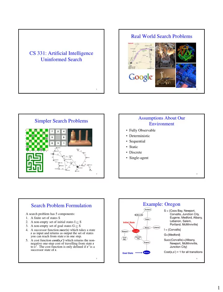
Example: Oregon

Corvallis Eugene Albany Lebanon Salem Newport Coos Bay McMinnville Portland Junction City Medford

S = {Coos Bay, Newport, Corvallis, Junction City, Eugene, Medford, Albany, Lebanon, Salem, Portland, McMinnville} I = {Corvallis} G={Medford} Succ(Corvallis)={Albany, Newport, McMinnville, Junction City} Cost(s,s’) = 1 for all transitions

Goal State Initial State

2

7

• Solution

Path from initial state to goal state

• Solution quality

Path cost (3 in this case)

• Optimal solution

Lowest path cost among all solutions (In this case, we found the optimal solution)

Results of a Search Problem

Junction City Corvallis Eugene Medford

8

Search Tree

Corvallis

Start with Initial State

9

Search Tree

Corvallis

Is initial state the goal?

• Yes, return solution
• No, apply Successor()

function

Newport McMinnville Albany Junction City

10

Search Tree

Corvallis

Apply Successor() function

Newport McMinnville Albany Junction City

These nodes have not been expanded yet. Call them the

• fringe. We’ll put them in a

queue. McMinnville Albany Junction City Newport Queue

11

Search Tree

Corvallis Newport McMinnville Albany Junction City

Albany Junction City Newport Portland Queue

Portland

Now remove a node from the queue. If it’s a goal state, return the solution. Otherwise, call Successor() on it, and put the results in the queue. Repeat.

Search Tree

Corvallis Newport McMinnville Albany Junction City

Albany Junction City Newport Portland Queue

Portland

Things to note:

• Order in which you expand nodes (in this

example, we took the first node in the queue)

• Avoid repeated states

3

13

Tree-Search Pseudocode

14

Tree-Search Pseudocode

Note: Goal test happens after we grab a node off the queue.

15

Tree-Search Pseudocode

Why are these parent node backpointers are important?

16

Uninformed Search

• No info about states other than generating

successors and recognizing goal states

• Later on we’ll talk about informed search –

can tell if a non-goal state is more promising than another

17

Evaluating Uninformed Search

• Completeness

Is the algorithm guaranteed to find a solution when there is one?

• Optimality

Does it find the optimal solution?

• Time complexity

How long does it take to find a solution?

• Space complexity

How much memory is needed to perform the search

18

Complexity

1. Branching factor (b) – maximum number of successors of any node 2. Depth (d) of the shallowest goal node 3. Maximum length (m) of any path in the search space Time Complexity: number of nodes generated during search Space Complexity: maximum number of nodes stored in memory

4

19

Uninformed Search Algorithms

• Breadth-first search
• Uniform-cost search
• Depth-first search
• Depth-limited search
• Iterative Deepening Depth-first Search
• Bidirectional search

20

Breadth-First Search

• Expand all nodes at a given depth before

any nodes at the next level are expanded

• Implement with a FIFO queue

21

Breadth First Search Example

A B E D C F G A B E D C F G Not yet reached Closed (expanded) nodes Open nodes (on the fringe) Current node to be expanded

22

Breadth First Search Example

A B E D C F G A B E D C F G Not yet reached Closed (expanded) nodes Open nodes (on the fringe) Current node to be expanded

23

Evaluating BFS

Complete? Optimal? Time Complexity Space Complexity

24

Evaluating BFS

Complete? Yes provided branching factor is finite Optimal? Time Complexity Space Complexity

5

25

Evaluating BFS

Complete? Yes provided branching factor is finite Optimal? Yes if step costs are identical Time Complexity Space Complexity

26

Evaluating BFS

Complete? Yes provided branching factor is finite Optimal? Yes if step costs are identical Time Complexity b+b2+b3+…+bd+(bd+1-b)= O(bd+1) Space Complexity

27

Evaluating BFS

Complete? Yes provided branching factor is finite Optimal? Yes if step costs are identical Time Complexity b+b2+b3+…+bd+(bd+1-b)= O(bd+1) Space Complexity O(bd+1)

Exponential time and space complexity make BFS impractical for all but the smallest problems

28

Uniform-cost Search

• What if step costs are not equal?
• Recall that BFS expands the shallowest node
• Now we expand the node with the lowest path cost
• Uses priority queues

Note: Gets stuck if there is a zero-cost action leading back to the same state. For completeness and optimality, we require the cost of every step to be ≥ 

29

Evaluating Uniform-cost Search

Complete? Optimal? Time Complexity Space Complexity

30

Evaluating Uniform-cost Search

Complete? Yes provided branching factor is finite and step costs ≥  for small positive  Optimal? Time Complexity Space Complexity

6

31

Evaluating Uniform-cost Search

Complete? Yes provided branching factor is finite and step costs ≥  for small positive  Optimal? Yes Time Complexity Space Complexity

32

Evaluating Uniform-cost Search

Complete? Yes provided branching factor is finite and step costs ≥  for small positive  Optimal? Yes Time Complexity O(b1+floor(C*/)) where C* is the cost of the optimal solution Space Complexity

33

Evaluating Uniform-cost Search

Complete? Yes provided branching factor is finite and step costs ≥  for small positive  Optimal? Yes Time Complexity O(b1+floor(C*/)) where C* is the cost of the optimal solution Space Complexity O(b1+floor(C*/)) where C* is the cost of the optimal solution

34

Depth-first Search

• Expands the deepest node in the current

fringe of the search tree

• Implemented with a LIFO queue

Depth-first Search Example

H I J K L M N O D E F G B C A H I J K L M N O D E F G B C A H I J K L M N O D E F G B C A H I J K L M N O D E F G B C A H I J K L M N O D E F G B C A H I J K L M N O D E F G B C A Not yet reached Expanded nodes on current path Expanded nodes with no descendants in the fringe (can be removed from memory) On fringe but unexpanded Current node to be expanded M Goal state

Depth-first Search Example

H I J K L M N O D E F G B C A H I J K L M N O D E F G B C A H I J K L M N O D E F G B C A H I J K L M N O D E F G B C A H I J K L M N O D E F G B C A H I J K L M N O D E F G B C A Not yet reached Expanded nodes on current path Expanded nodes with no descendants in the fringe (can be removed from memory) On fringe but unexpanded Current node to be expanded M Goal state

7

37

Evaluating Depth-first Search

Complete? Optimal? Time Complexity Space Complexity

38

Evaluating Depth-first Search

Complete? Yes on finite graphs. No if there is an infinitely long path with no solutions. Optimal? Time Complexity Space Complexity

39

Evaluating Depth-first Search

Complete? Yes on finite graphs. No if there is an infinitely long path with no solutions. Optimal? No (Could expand a much longer path than the optimal one first) Time Complexity Space Complexity

40

Evaluating Depth-first Search

Complete? Yes on finite graphs. No if there is an infinitely long path with no solutions. Optimal? No (Could expand a much longer path than the optimal one first) Time Complexity O(bm) Space Complexity

41

Evaluating Depth-first Search

Complete? Yes on finite graphs. No if there is an infinitely long path with no solutions. Optimal? No (Could expand a much longer path than the optimal one first) Time Complexity O(bm) Space Complexity O(bm)

42

Depth-limited Search

• Solves infinite path problem by using

predetermined depth limit l

• Nodes at depth l are treated as if they have

no successors

• Can use knowledge of the problem to

determine l (but in general you don’t know this in advance)

8

43

Evaluating Depth-limited Search

Complete? Optimal? Time Complexity Space Complexity

44

Evaluating Depth-limited Search

Complete? No (If shallowest goal node beyond depth limit) Optimal? Time Complexity Space Complexity

45

Evaluating Depth-limited Search

Complete? No (If shallowest goal node beyond depth limit) Optimal? No (If depth limit > depth of shallowest goal node and we expand a much longer path than the optimal one first) Time Complexity Space Complexity

46

Evaluating Depth-limited Search

Complete? No (If shallowest goal node beyond depth limit) Optimal? No (If depth limit > depth of shallowest goal node and we expand a much longer path than the optimal one first) Time Complexity O(bl) Space Complexity

47

Evaluating Depth-limited Search

Complete? No (If shallowest goal node beyond depth limit) Optimal? No (If depth limit > depth of shallowest goal node and we expand a much longer path than the optimal one first) Time Complexity O(bl) Space Complexity O(bl)

48

Iterative Deepening Depth-first Search

• Do DFS with depth limit 0, 1, 2, … until a

goal is found

• Combines benefits of both DFS and BFS

9

49

Iterative Deepening Depth-first Search Example

A A

Limit = 0

B C A B C A

Limit = 1

B C A B C A

Limit = 2

D E F G B C A D E F G B C A D E F G B C A D E F G B C A D E F G B C A D E F G B C A D E F G B C A D E F G B C A

50

IDDFS Example

Limit = 3

H I J K L M N O D E F G B C A H I J K L M N O D E F G B C A H I J K L M N O D E F G B C A H I J K L M N O D E F G B C A H I J K L M N O D E F G B C A H I J K L M N O D E F G B C A

51

IDDFS Example

H I J K L M N O D E F G B C A H I J K L M N O D E F G B C A H I J K L M N O D E F G B C A H I J K L M N O D E F G B C A H I J K L M N O D E F G B C A H I J K L M N O D E F G B C A

Limit = 3 (Continued)

52

Evaluating Iterative Deepening Depth-first Search

Complete? Optimal? Time Complexity Space Complexity

53

Evaluating Iterative Deepening Depth-first Search

Complete? Yes provided branching factor is finite Optimal? Time Complexity Space Complexity

54

Evaluating Iterative Deepening Depth-first Search

Complete? Yes provided branching factor is finite Optimal? Yes if the path cost is a nondecreasing function of the depth of the node Time Complexity Space Complexity

10

55

Evaluating Iterative Deepening Depth-first Search

Complete? Yes provided branching factor is finite Optimal? Yes if the path cost is a nondecreasing function of the depth of the node Time Complexity O(bd) Space Complexity

56

Evaluating Iterative Deepening Depth-first Search

Complete? Yes provided branching factor is finite Optimal? Yes if the path cost is a nondecreasing function of the depth of the node Time Complexity O(bd) Space Complexity O(bd)

57

Isn’t Iterative Deepening Wasteful?

• Actually, no! Most of the nodes are at the bottom

level, doesn’t matter that upper levels are generated multiple times.

• To see this, add up the 4th column below:

Depth # of nodes # of times generated Total # of nodes generated at depth d 1 b d (d)b 2 b2 d-1 (d-1)b2 : : : : d bd 1 (1)bd

58

Is Iterative Deepening Wasteful?

Total # of nodes generated by iterative deepening: (d)b + (d-1)b2 +… + (1)bd = O(bd+1) Total # of nodes generated by BFS: b + b2 +… + bd + bd+1 - b = O(bd+1) In general, iterative deepening is the preferred uninformed search method when there is a large search space and the depth of the solution is not known

59

Bidirectional Search

• Run one search forward from the initial state
• Run another search backward from the goal
• Stop when the two searches meet in the middle

60

Bidirectional Search

• Needs an efficiently computable

Predecessor() function

• What if there are several goal states?

– Create a new dummy goal state whose predecessors are the actual goal states

• Difficult when the goal is an abstract

description like “no queen attacks another queen”

11

61

Evaluating Bidirectional Search

Complete? Optimal? Time Complexity Space Complexity

62

Evaluating Bidirectional Search

Complete? Yes provided branching factor is finite and both directions use BFS Optimal? Time Complexity Space Complexity

63

Evaluating Bidirectional Search

Complete? Yes provided branching factor is finite and both directions use BFS Optimal? Yes if the step costs are all identical and both directions use BFS Time Complexity Space Complexity

64

Evaluating Bidirectional Search

Complete? Yes provided branching factor is finite and both directions use BFS Optimal? Yes if the step costs are all identical and both directions use BFS Time Complexity O(bd/2) Space Complexity

65

Evaluating Bidirectional Search

Complete? Yes provided branching factor is finite and both directions use BFS Optimal? Yes if the step costs are all identical and both directions use BFS Time Complexity O(bd/2) Space Complexity O(bd/2) (At least one search tree must be kept in memory for the membership check)

66

Avoiding Repeated States

• Tradeoff between space and time!
• Need a closed list which stores every expanded

node (memory requirements could make search infeasible)

• If the current node matches a node on the closed

list, discard it (ie. discard the newly discovered path)

• We’ll refer to this algorithm as GRAPH-SEARCH
• Is this optimal? Only for uniform-cost search or

breadth-first search with constant step costs.

12

67

GRAPH-SEARCH

68

Things You Should Know

• How to formalize a search problem
• How BFS, UCS, DFS, DLS, IDS and

Bidirectional search work

• Whether the above searches are complete

and optimal plus their time and space complexity

• The pros and cons of the above searches