Ray Tracing Ray Tracing Classical geometric optics technique - PDF document

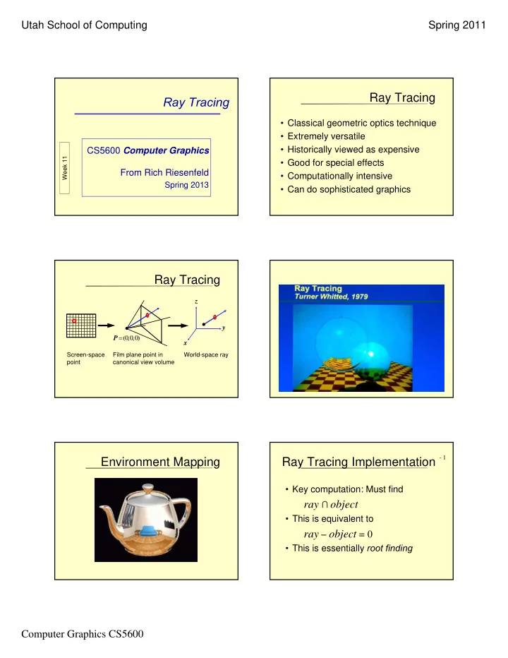
Utah School of Computing Spring 2011 Ray Tracing Ray Tracing • Classical geometric optics technique • Extremely versatile • Historically viewed as expensive CS5600 Computer Graphics Week 11 • Good for special effects From Rich Riesenfeld • Computationally intensive Spring 2013 • Can do sophisticated graphics Ray Tracing z y  P (0,0,0) x Screen-space Film plane point in World-space ray point canonical view volume - 1 Environment Mapping Ray Tracing Implementation • Key computation: Must find ray ∩ object • This is equivalent to ray – object = 0 • This is essentially root finding Computer Graphics CS5600

Utah School of Computing Spring 2011 - 2 - 3 Ray Tracing Implementation Ray Tracing Implementation • Ray is often represented parametrically, • RT’ing used for spectacular images r ( t ) = t ( P - E ) , • RT’ing maps naturally to recursion so we seek, • RT’ing is trivially parallelized r ( t ) ∩ F ( x,y,z ) • RT’ing has robustness problems • Problem requires intersection of parametric ray with some kind of surface • RT’ing has aliasing problems • Ray Tracing maps easily onto recursion - 1 - 2 Ray Tracing Ray Tracing Three ( nonexclusive ) phenomena • Forward ray tracing: E ( S  DL follow when ray intersects object: 1. Reflect (specularity) • Backward ray tracing: L ( S  DE 2. Pass through (transparency) 3. Stop (diffuse - look for light vector • What is the difference? and calculate proper value) Ray Tracing (ternary) Tree Ray Tracing (fwd) Diffuse Often a combination of all three occur at each node to model sophisticated effects Ray impinges Diffuse Diffuse Transmit Reflect Stop (Transparent (specular) (Diffuse) /translucent) Diffuse Computer Graphics CS5600

Utah School of Computing Spring 2011 Ray Tracing (fwd) Ray Tracing (fwd) Diffuse Diffuse Diffuse Diffuse Diffuse Diffuse Diffuse Diffuse RT’ing Indirect Light (bkwd) RT’ing Indirect Light (bkwd) Diffuse Diffuse x Specular Specular Diffuse Diffuse Diffuse Diffuse RT’ing Indirect Light (bkwd) Ray Tracing Growth Diffuse • Tree can grow extremely fast, with high exponential fan out Specular Diffuse • Fancy rays can have many cross- section geometries; not necessary a line with 0-cross-section • Need to bound tree depth & fanout Diffuse Computer Graphics CS5600

Utah School of Computing Spring 2011 Returning to Ray Tracing z y  P (0,0,0) x Screen-space point Film plane point in World-space ray canonical view volume Returning to Ray Tracing Returning to Ray Tracing z z s e e y y x x World-space ray World-space ray Returning to Ray Tracing Returning to Ray Tracing z z e e - - s s s s e e y y ray(t)=e + t (s – e) ray(t)=e + t (s – e) x x t = 0? World-space ray World-space ray t = s? t < 0 ? Computer Graphics CS5600

Utah School of Computing Spring 2011 Returning to Ray Tracing How to chose initial ray? z e t 2 - s t 1 s e y ray(t)=e + t (s – e) x t < 0 ? World-space ray t 1 < t 2 Rays through the pixels Orthographic Perspective Returning to Ray Tracing z uvw coordinate system e - s Origin is e  i 0 . 5   u l ( r l )  s s n x e  j 0 . 5   v b ( t b ) y  s n y  ray(t)=e + t (s – e) w near s x World-space ray Computer Graphics CS5600

Utah School of Computing Spring 2011 Computing Areas: Recall Barycentric Coords: Areas ฀   Area PBC ฀   Area ABDC AB AC ฀ C Area ABC ฀   1 Area ABC AB AC ฀ 2   Area PCA ฀ A Area ABC C ฀   D Area PAB ฀ B P ABC Area A B Barycentric Coords: Areas Isoparametric lines C C Then,     , , 0, constant        1, A A  and, P      A B C B B P P Extended Barycentric Coords Extended Barycentric Coords C C Can use Then,         , , 0 ? , , 0, A A       1, for test of P  and, P B B P P ฀ ABC outside      ? A B C P can be outside triangle if P can be outside triangle, coord’s allowed to go but in it plane, if coord’s can be negative. negative. Computer Graphics CS5600

Utah School of Computing Spring 2011 Algorithm for Computing Algorithm for Computing - 1 - 2 Barycentric Coords of P Barycentric Coords of P C C 2. Compute all 1. As indicated, areas using assign an ฀ ฀ PAB PBC , A A orientation to ฀ and PCA ฀ ABC Orientation is B P B important! P Algorithm for Computing Algorithm for Computing - 3 - 4 Barycentric Coords of P Barycentric Coords of P C 3. Compute all areas using cross products in the following manner,    AB BC 2 Area big A    PB BC 2 Area  B   Note this works  PC CA P 2 Area  equally for P outside    PA AB 2 Area  Algorithm for Computing Algorithm for Computing - 5 - 6 Barycentric Coords of P Barycentric Coords of P    4. Now compute ratios for , , 5. Now compute sign of area. In or out ? Look at dot product of area vectors! P is  PB BC   2 Area     in if same sign, i.e., positive; out , outwise.  2 Area AB BC big   PC CA   2 Area       ฀  sign ( PB BC ) ( AB BC ) Sign    2 Area AB BC big     ฀   sign ( PC CB ) ( AB BC ) Sign PA AC   2  Area          2 Area AB BC ฀  sign ( PA AC ) ( AB BC ) Sign big  Computer Graphics CS5600

Utah School of Computing Spring 2011 - 1 Applet Recall Cramer’s Rule       m m m x y   1 1 Universität Karlsruhe (TH) 11 12 13       m m m x  y Let, 2 2 Geometrische Datenverarbeitung:       21 22 23   x y m m m       3 3 31 32 33  Mx y That is, < http://i33www.ira.uka.de/applets/mocca/html/noplugin/inhalt.html > m m m 11 12 13   M m m m det( M ) and, 21 22 23 m m m 31 32 33 - 2 Ray Intersect Parametic Object Recall Cramer’s Rule Then,    Let ( , ) S ( , ), ( , ), ( , ) u v f u v g u v h u v y m m m y m 1 12 13 11 1 13 be a parametrically defined object. 1 1   x y m m ; x m y m ; 2 22 23 21 2 23 1 2 M M Componentwise, this means, y m m m y m 3 32 33 31 3 33   e td f u v ( , ) and, x x m m y   e td g u v ( , ) 11 12 1 1  y y x m m y 2 1 2 2 2 3 M   e td h u v ( , ) m m y 31 32 3 z z Ray Tracing Barycentric Coords: Areas Then, C d z     d , , 0,       e 1, e y A  and, P x      A B C B P Computer Graphics CS5600

Utah School of Computing Spring 2011 t  ฀ Ray Intersect Parametic Object p ( ) ABC Solving for       , )       Let ( , ) S u v f u v g u v h u v ( , ), ( , ), ( , ) P ( , A B C C be a parametrically defined object.  p ( ) t A td Componentwise, this means,  e t d   e td f u v ( , ) x x   e td g u v ( , ) e y y B   e td h u v ( , ) z z ray  ฀ ray  ฀ Shirley’s Method - 1 Shirley’s Method - 2   We can think of this form as Let ( ) p t e t d be a ray, and establishing the origin at , and A define the plane as              P ( , , ) A B C , using basis vectors ( B A ),( C A ) ฀     to span the plane of ABC :            or, ( , ) P (1 ) A B C          P A B A C A ( , ) ( ) ( )        A B A C A ( ) ( ) ray  ฀ ray  ฀ Shirley’s Method - 3 Shirley ’ s Method - 4   Where do ray ( ) p t e t d , and In matrix form plane defined as          A B A C d A e ( ) ( ) t         P ( , , ) A B C , intersect?                A ( B A ) ( C A ) e t d      ( A B ) ( A C ) d A e           A e = ( B A ) ( C A ) t d   t         ( A B ) ( A C ) t d A e Computer Graphics CS5600