Ramin Raziperchikolaei Electrical Engineering and Computer Science - - PowerPoint PPT Presentation

ramin raziperchikolaei electrical engineering and
SMART_READER_LITE
LIVE PREVIEW

Ramin Raziperchikolaei Electrical Engineering and Computer Science - - PowerPoint PPT Presentation

An Ensemble Diversity Approach to Binary Hashing Ramin Raziperchikolaei Electrical Engineering and Computer Science University of California, Merced http://eecs.ucmerced.edu Joint work with Miguel A. Carreira-Perpi n an Large


slide-1
SLIDE 1

An Ensemble Diversity Approach to Binary Hashing

Ramin Raziperchikolaei Electrical Engineering and Computer Science University of California, Merced http://eecs.ucmerced.edu Joint work with Miguel ´

  • A. Carreira-Perpi˜

n´ an

slide-2
SLIDE 2

Large Scale Image Retrieval

Searching a large database for images that are closest to a query. This is the k nearest neighbors problem on N vectors in RD with large N and D.

Query Database Top retrieved image

  • p. 1
slide-3
SLIDE 3

Binary Hash Functions

A binary hash function h takes as input a high-dimensional vector x ∈ RD and maps it to an b-bit vector z = h(x) ∈ {0, 1}b. ❖ Main goal: preserve neighbors, i.e., assign (dis)similar codes to (dis)similar patterns. ❖ Hamming distance computed using XOR and then counting. 1 1 1 1 1 1 1 1 1 1

Image Binary Codes

XOR

Hamming Distance = 3

  • p. 2
slide-4
SLIDE 4

Binary Hash Functions in Large Scale Image Retrieval

Scalability: we have millions or billions of high-dimensional images. ❖ Time complexity: O(Nb) instead of O(ND) with small constants. ✦ Bit operations to compute Hamming distance instead of floating point operations to compute Euclidean distance. ❖ Space complexity: O(Nb) instead of O(ND) with small constants. We can fit the binary codes of the entire dataset in memory, further speeding up the search. Ex: N = 1 000 000 points, D = 300 and b = 32: Space Time Original space 1.2 GB 20 ms Hamming space 4 MB 30 µs

  • p. 3
slide-5
SLIDE 5

Affinity-Based Objective Functions

Affinity matrix W determines similar and dissimilar pairs of points among the points in the training set X = (x1, . . . , xN), for example: wnm =    1 xn and xm are similar −1 xn and xm are dissimilar We do not know xn and xm are similar if: label(xn) = label(xm) supervised dataset xn − xm < ǫ unsupervised dataset Learn hash function h(·) ∈ {0, 1}b by minimizing the affinity-based

  • bjective function:

min L(h) =

N

  • n,m=1

L(h(xn), h(xm); wnm) where h(xn) ∈ {0, 1}b L(·) is a loss function that compares the codes for two images with the ground-truth value wnm.

  • p. 4
slide-6
SLIDE 6

Optimizing Affinity-Based Objective Functions

Many hashing papers use affinity based objective function: Laplacian loss (Spectral Hashing (Weiss et al. 2008), Hashing with Graphs (Liu et al. 2011), etc.): L(h) =

N

  • n,m=1

wnm h(xn) − h(xm)2 s.t. h(X)Th(X) = NI h(X)T1 = 0. KSH Loss (Supervised Hashing with Kernels (Liu et al. 2012), Two-Step Hashing (Lin et al. 2013),

etc.):

L(h) =

N

  • n,m=1

(h(xn)Th(xm) − b wnm)2 Since the output of the hash function is binary, the objective function is nonsmooth and difficult to optimize. All the one bit hash functions, h = [h1, . . . , hb], are coupled to force them to be different from each other. This further complicates the

  • ptimization: Optimization takes a long time, it limits the number of points and bits in training, etc.

The goal of Most binary hashing wroks is to propose a new objective function and an approximate way to optimize it. We propose a different approach to learn good hash functions.

  • p. 5
slide-7
SLIDE 7

Training Binary Hash Functions Independently

We propose to optimize each 1-bit hash function independently from the rest. This gives us several advantages: ❖ Optimization simplifies greatly: we deal with b independent problem each over N

binary codes rather than 1 problem with with Nb binary codes.

❖ This will lead to faster training and better accuracy. ❖ Training can be done in parallel. But, how to make sure that the b hash functions are different from each

  • ther and their combination results in good retrieval?

We will introduce diversity in a different way: We use diversity techniques from the ensemble learning literature.

  • p. 6
slide-8
SLIDE 8

A Single Bit Affinity-based Objective Function

Independent Laplacian Hashing (ILH): We focus on the following objective function to learn a 1-bit hash function h(·): L(h) =

N

  • n,m=1

wnm(h(xn) − h(xm))2 We can use existing algorithms for optimizing affinity-based objective functions, which becomes particularly effective with our 1-bit objective

  • functions. For example:

❖ (1) Relax the binary constraints, (2) solve the problem assuming that the hash functions are continuous and (3) truncate the results to achieve the binary codes. ❖ (1) Replace the hash functions by binary codes zn = h(xn), (2) find the binary codes using binary

  • ptimization techniques like Graph-Cut, and (3) Learn hash functions by training classifiers from input

to the binary codes.

We show that we can avoid trivial solutions by injecting diversity into each hash function’s training using techniques inspired from classifier ensemble learning.

  • p. 7
slide-9
SLIDE 9

Adding Diversity with Ensemble Learning Techniques

If we optimize the same objective function b times, we get b identical hash functions and we gain nothing over a single hash function. A similar problem arises in ensemble learning: we want to train several classifiers on the same training set. If the classifiers are all equal, we gain nothing over a single classifier. We consider the following diversity mechanisms from the ensemble learning literature: ❖ Different initializations (ILHi): Each hash function is initialized randomly, which results

in different local optima for different hash functions.

❖ Different training sets (ILHt): Each hash function uses a training set of N points that is

different from the other hash functions.

❖ Different feature subsets (ILHf): Each hash function is trained on a random subset of

1 ≤ d ≤ D features.

  • p. 8
slide-10
SLIDE 10

Advantages of Independent Laplacian Hashing

❖ b binary optimizations over N binary variables each is generally easier than one binary optimization over bN variables. ❖ Training the b functions can be parallelized perfectly. ❖ To get the solution for b + 1 bits we just need to take a solution with b bits and add one more bit. ✦ This is helpful for model selection. How many bits do we need in binary hashing? We can maximize the precision on a test set

  • ver b (cross-validation).

✦ Computationally easy: simply keep adding bits until the test precision stabilizes. ❖ For ILHf, both the training and test time are lower than if using all D features for each hash function. The test runtime for a query is d/D smaller.

  • p. 9
slide-11
SLIDE 11

Experiments: Diversity Mechanisms with ILH

32 bits 64 bits 128 bits

precision

0.2 0.5 1 2 x 10

4

30 35 40 45 ILHi ILHt ILHf ILHitf KSH

N

0.2 0.5 1 2 x 10

4

30 35 40 45 ILHi ILHt ILHf ILHitf KSH

N

0.2 0.5 1 2 x 10

4

30 35 40 45 ILHi ILHt ILHf ILHitf KSH

N

CIFAR dataset, N = 58 000 training/ 2 000 test images, D = 320 SIFT features.

As a device to make the hash functions different and produce good retrival, the diversity mechanisms work as well as or quite better than using optimization. The clearly best diversity mechanism is ILHt, which works better than the other mechanisms, even when combined with them, and significantly better than KSH.

  • p. 10
slide-12
SLIDE 12

Preformance as a Function of Number of Bits

precision

40 80 120 160 200 10 20 30 40 45

ILHt KSH LSH tPCA

number of bits b

For KSH the variance is large (compared to ILHt) and the precision barely increases after b = 80. For ILHt, the precision increases nearly monotonically and continues increasing beyond b = 200 bits.

  • p. 11
slide-13
SLIDE 13

ILHt Compared with Other Binary Hashing Methods

b = 32 b = 64 b = 128

precision

500 600 700 800 900 1000 20 25 30 35 40 45 ILHt KSHcut KSH STH ITQ−CCA LSH BRE

k

500 600 700 800 900 1000 20 25 30 35 40 45

k

500 600 700 800 900 1000 20 25 30 35 40 45

k

precision

20 40 60 80 100 10 20 30 40 45 ILHt KSHcut KSH STH ITQ−CCA LSH BRE

recall

20 40 60 80 100 10 20 30 40 45

recall

20 40 60 80 100 10 20 30 40 45

recall

CIFAR dataset, N = 58 000 training/ 2 000 test images, D = 320 SIFT features. Groundtruth: points with the same labels as the query

ILHt beats state-of-the-art methods, particularly as the number of bits b increases.

  • p. 12
slide-14
SLIDE 14

Conclusion

❖ Most hashing papers try to learn good hash functions by minimizing a sophisticated affinity-based objective function that couples all the binary codes. This results in a very difficult, slow optimization. ❖ This is not necessary! We have shown that the hash functions can be trained independently: ✦ Much simpler optimization. Over N binary codes instead of Nb. ✦ Training is fast and parallel. b 1-bit hash functions trained independently. ✦ Performance is competitive or even quite better than the state-of-the-art. ❖ We need diversity techniques to avoid trivial solutions:

✦ ILHi: different initialization. ✦ ILHf: different sets of features in training hash functions. ✦ ILHt: different subsets of points and works best. Partly supported by NSF award IIS–1423515.

  • p. 13
slide-15
SLIDE 15

Experiments: Diversity Mechanisms with ILH (Cont.)

ILHf ILHitf ILHt Incremental ILHt

precision

0.01 0.2 0.4 0.6 0.8 1 10 20 30 40 50 60 70 80

d/D b = 32 b = 64 b = 128

0.01 0.2 0.4 0.6 0.8 1 10 20 30 40 50 60 70 80

d/D b = 32 b = 64 b = 128

32 64 128 10 20 30 40 50 60 70 80

disjoint random sampling bootsrtap number of bits b

40 80 120 160 200 10 20 30 40 50 60 70 80

ILHt KSHcut tPCA LSH number of bits b

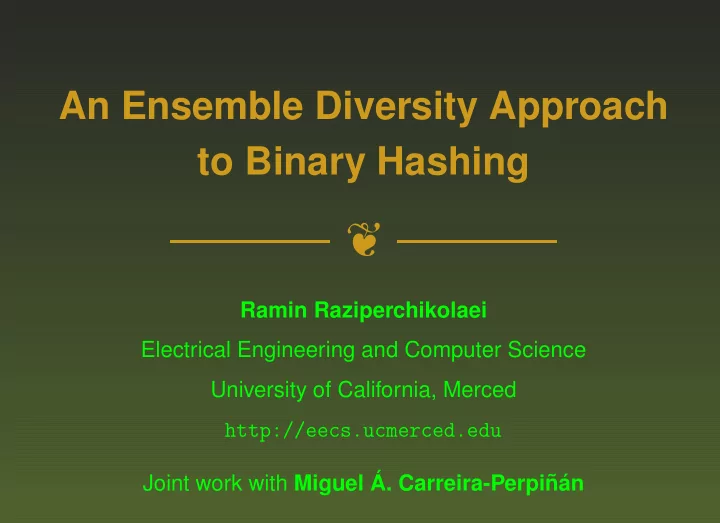
INFMNIST dataset, N = 1 000 000 training/ 2 000 test images, D = 784 raw pixel features. (panels 1–2) shows the results in ILHf of varying the number of features 1 ≤ d ≤ D used by each hash

  • function. The highest precision is achieved with a proportion d/D ≈ 30% for ILHf.

(panel 3) shows the results of using bootstrapped (samples with replacement from 5 000 points) instead of disjoint training sets for ILHt. As expected, the latter is consistently better. (panel 4) shows the precision (in the test set) as a function of the number of bits b for ILHt, where the solution for b + 1 bits is obtained by adding a new bit to the solution for b. ❖ For KSHcut the variance is large (compared to ILHt) and the precision barely increases after b = 30. ❖ For ILHt, the precision increases nearly monotonically and continues increasing beyond b = 200 bits.

  • p. 14
slide-16
SLIDE 16

Comparison with Other Binary Hashing Methods

b = 32 b = 64 b = 128 precision

6000 7000 8000 9000 10000 10 20 30 40

ILHt KSHcut KSH STH ITQ BA tPCA SH LSH BRE

k

6000 7000 8000 9000 10000 10 20 30 40

k

6000 7000 8000 9000 10000 10 20 30 40

k

precision

20 40 60 80 100 20 40 60 80

ILHt KSHcut KSH STH ITQ BA tPCA SH LSH BRE

recall

20 40 60 80 100 20 40 60 80

recall

20 40 60 80 100 20 40 60 80

recall

FLICKR dataset, N = 1 000 000 training/ 10 000 test images, D = 150 edge histogram features. Groundtruth: First K = 10 000 nearest neighbors of the query in the original space. ILHt beats state-of-the-art methods, particularly as the number of bits b increases.

  • p. 15