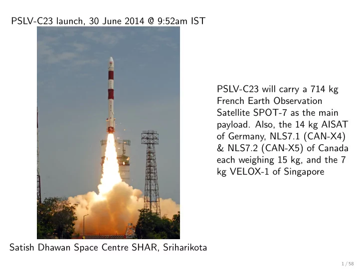
PSLV-C23 launch, 30 June 2014 @ 9:52am IST PSLV-C23 will carry a 714 - PowerPoint PPT Presentation

PSLV-C23 launch, 30 June 2014 @ 9:52am IST PSLV-C23 will carry a 714 kg French Earth Observation Satellite SPOT-7 as the main payload. Also, the 14 kg AISAT of Germany, NLS7.1 (CAN-X4) & NLS7.2 (CAN-X5) of Canada each weighing 15 kg, and the 7 kg VELOX-1 of Singapore Satish Dhawan Space Centre SHAR, Sriharikota 1 / 58

Aryabhatta, India’s first satellite Launched on 19 April 1975, by KOSMOS-3M (Soviet-Union) 2 / 58

DG-KFVS schemes for convection-diffusion equations Praveen. C Center for Applicable Mathematics Tata Institute of Fundamental Research Bangalore-560065, India http://math.tifrbng.res.in/~praveen Dept. of Mathematics University of W¨ urzburg 30 June, 2014 3 / 58

Compressible Navier-Stokes model • Mass conservation equation ∂ρ ∂t + ∇ · ( ρ u ) = 0 • Momentum equation ∂ ∂t ( ρ u ) + ∇ · ( pI + ρ uu ) = ∇ · τ • Energy conservation ∂E ∂t + ∇ · ( E + p ) u = ∇ · ( u · τ ) + ∇ · q 4 / 58

Compressible Navier-Stokes model • Equation of state: ideal gas γ − 1 + 1 p 2 ρ | u | 2 , E = γ > 1 • Constitutive laws τ ij = µ ( ∂ i u j + ∂ j u i ) − 2 3 µ ( ∂ k u k ) δ ij , q i = − κ∂ i T • System of conservation laws ∂U ∂t + ∂ F i ( U ) + ∂ G i ( U, ∇ U ) = 0 ∂x i ∂x i 5 / 58

Flow over NACA0012 airfoil: M = 0 . 85 , α = 1 Pressure 5 Kinetic meshless method 6 / 58

Flow through scramjet intake Density Kinetic meshless method 7 / 58

Kinetic description of gases • Gas composed of many molecules • Describe state of gas by a velocity distribution function x ∈ R 3 , v ∈ R 3 f ( x, v, t ) , • Number density of gas molecules � n ( x, t ) = R 3 f ( x, v, t )d v =: � f � • Mass density ρ ( x, t ) = mn ( x, t ) , m = mass of one molecule We will assume that f is rescaled to give mass density, � f � = ρ . 8 / 58

Kinetic description of gases • Basic conserved quantities ρ = � f �   1 ρu = � vf � U = � ψf � , ψ = v   1 2 | v | 2 � ( v 2 / 2) f � ρe = • Evolution of f governed by Boltzmann equation ∂f ∂t + v · ∇ f = J ( f, f ) • Collisions do not change mass, momentum, energy � ψJ ( f, f ) � = 0 ψ are the only collisional invariants. 9 / 58

Kinetic description of gases • Equilibrium distribution: Maxwell-Boltzmann distribution function f = g = exp( a + b · v + c | v | 2 ) J ( f, f ) = 0 = ⇒ or in the more familiar form � 3 / 2 � β 1 − β | v − u | 2 � � g ( v ) = ρ exp , β = π 2 RT • Moments of g lead to Euler equations U = � ψg � , F i = � v i ψg � � ∂g ∂g � ∂U ∂t + ∂F i ∂t + v i = 0 = ⇒ = 0 ∂x i ∂x i Construct numerical scheme for Boltzmann eqn (linear convection eqn), average over all velocities to obtain scheme for Euler equation 10 / 58

Kinetic model for convection equation The scalar convection equation u t + cu x = 0 (1) can be obtained from a “Maxwell-Boltzmann” distribution � β � − β ( v − c ) 2 � g ( v, u ) = u π exp (2) since � g � = u and � vg � = cu The ”Boltzmann equation” for the distribution function is obtained by differentiating equation (2) � β � − β ( v − c ) 2 � g t + vg x = ( v − c ) u x π exp =: Q (3) Note that the moment of the collision term Q is zero, � Q � = 0 so that taking moments of equation (3) gives us the convection equation (1). 11 / 58

Kinetic numerical flux Discontinuous solution in a finite volume or finite element method u − j +1 / 2 u ± ( x ) = lim u + ǫ ց 0 u ( x ∓ ǫ ) j +1 / 2 j − 1 / 2 I j j + 1 / 2 I j +1 j + 3 / 2 In the kinetic model, molecules carry information due to their streaming motion. This allows us to use the upwind principle to approximate the velocity distribution function at x j + 1 2 based on the sign of the molecular velocity as g ( v, u + � 2 ) v > 0 j + 1 g j + 1 2 = g ( v, u − 2 ) v < 0 j + 1 12 / 58

Kinetic numerical flux Numerical flux function 2 � = F + ( u + 2 ) + F − ( u − 2 ) =: F ( u + 2 , u − F j + 1 2 = � vg j + 1 2 ) j + 1 j + 1 j + 1 j + 1 The split fluxes are obtained by integrating over half velocity spaces, and are given by � ∞ � 0 F ± ( u ) = cuA ± + uB ± F + ( u ) = F − ( u ) = vg d v, vg d v, 0 −∞ where A ± = 1 1 B ± = ± 2 √ πβ exp( − s 2 ) , � 2[1 ± erf( s )] , s = c β • F + is due to all molecules moving to the right ( v > 0 ) while the flux F − is due to all molecules moving to the left ( v < 0 ) • F ( u − , u + ) is consistent, i.e., F ( u, u ) = cu and is obviously a smooth function of u . 13 / 58

Kinetic numerical flux • The split flux F + ( u ) is an increasing function of u while F − ( u ) is a decreasing function. Hence the numerical flux F ( u − , u + ) is a monotone flux. • Central flux with dissipation F ( u + , u − ) = 1 2( cu + + cu − ) + 1 2 D ( u + − u − ) (4) where 1 √ πβ exp( − s 2 ) > 0 D = c erf( s ) + • In the limit of β → ∞ , D → | c | � cu + , c > 0 F ( u + , u − ) = cu − , c < 0 14 / 58

DG scheme for convection equation N � Ω = I j , I j = [ x j − 1 2 , x j + 1 2 ] , j = 1 , . . . , N j =1 The DG method uses the broken space of polynomials of degree k V k φ ∈ L 2 (Ω) : φ | I j ∈ P k ( I j ) � � h = Multiply equation (1) by a test function φ h ∈ V k h and integrate over element I j � � φ h ∂ t u h dx − cu h ∂ x φ h dx I j I j 2 φ h ( x + 2 φ h ( x − + F ( u h ) j + 1 2 ) − F ( u h ) j − 1 2 ) = 0 j + 1 j − 1 Use numerical flux at the element interface 2 = F ( u + 2 , u − F ( u h ) j + 1 2 ) j + 1 j + 1 15 / 58

DG scheme for convection equation If we take φ h = u h and sum over all elements, we obtain the energy equation N N 1 d � dt � u h � 2 − � � cu h ∂ x u h dx + F ( u h ) j + 1 2 � u h � j + 1 2 = 0 (5) 2 I j j =1 j =1 where we have defined the inter-element jump in the solution by 2 := u h ( x + 2 ) − u h ( x − � u h � j + 1 2 ) j + 1 j + 1 After some simple manipulations, the energy equation can be written as N 1 d t � u h � 2 + 1 d � � u h � 2 2 D 2 = 0 j + 1 2 j =1 and hence the DG scheme is stable in energy norm for any degree of basis functions. 16 / 58

Kinetic model for convection diffusion equation Consider the linear convection-diffusion equation u t + cu x = µu xx or u t + ( cu − µu x ) x = 0 , µ > 0 (6) Kinetic formulation using the Boltzmann equation with BGK model f t + vf x = g − f (7) τ R τ R is relaxation time scale towards local equilibrium distribution g . Chapman-Enskog expansion f = f 0 + τ R f 1 + τ 2 R f 2 + . . . (8) Substituting this in equation (7) and collecting terms with the same coefficient of τ R , we get f 0 = g, f 1 = − ( g t + vg x ) The first two terms constitute the Chapman-Enskog distribution function � β f ce = f 0 + τ R f 1 = [ u − τ R ( v − c ) u x ] − β ( v − c ) 2 � � π exp (9) 17 / 58

Kinetic model for convection diffusion equation Upon taking moments of this distribution function, we obtain � vf ce � = cu − τ R � f ce � = u, 2 β u x In order to recover the correct flux of equation (6), we have to choose � vf ce � = cu − µu x τ R = 2 βµ = ⇒ Since f ce is a truncated solution in the Chapman-Enskog expansion it does not satisfy equation (7). We can derive an equation for f ce by differentiating equation (9) f ce t + vf ce x = � � β � ( v − c ) u x + ( µ − τ R ( v − c ) 2 ) u xx − τ R µ ( v − c ) u xxx � − β ( v − c ) 2 � π exp =: Q Upon taking moments of this equation, the right hand side vanishes, i.e., � Q � = 0 and we obtain the convection-diffusion equation (6). 18 / 58

Flux vector splitting F = cu x − µu x Split fluxes due to positive and negative velocity particles � v ± | v | � F ± = = ( cu − µu x ) A ± + uB ± f ce 2 Numerical flux function F ( u + , u − ) = F + ( u + ) + F − ( u − ) = F c ( u + , u − ) + F d ( u + x , u − x ) where the convective flux F c is identical to equation (4), while the dissipative flux is given by x A + − µu − x A − =: F + x , u − x ) + F − d ( u − F d ( u + x ) = − µu + d ( u + x ) 19 / 58

DG scheme for convection-diffusion equation The DG discretization of equation (6) is obtained by multiplying it by a test function φ h and integrating over any element I j � � � φ h ∂ t u h d x − cu h ∂ x φ h d x + µ ( ∂ x u h )( ∂ x φ h )d x (10) I j I j I j 2 φ h ( x + 2 φ h ( x − + F ( u h ) j + 1 2 ) − F ( u h ) j − 1 2 ) = 0 j + 1 j − 1 In the above equation, the inter-element flux is approximated by the kinetic numerical flux which is defined as F ( u h ) = F c ( u + h , u − h ) + F d ( ∂ x u + h , ∂ x u − h ) and it includes both convective and diffusive fluxes. 20 / 58

Test Case We will consider the convection-diffusion equation (6) in the domain ( − 1 , +1) together with the initial condition u ( x, 0) = − sin( πx ) (11) and periodic boundary conditions. The exact solution to this problem is given by u ( x, t ) = − exp( − µπ 2 t ) sin( π ( x − ct )) (12) Test Case 1 2 µ 0.001 1 t f 30 0.5 Table : Parameters for the test case based on convection-diffusion equation (6) 21 / 58