Protein Docking and 3D Ligand-Based Virtual Screening Modeling - - PowerPoint PPT Presentation

Protein Docking and 3D Ligand-Based Virtual Screening Part 2 Dave Ritchie Orpailleur Team INRIA Nancy – Grand Est Modeling Protein Flexibility Using Elastic Network Models

• ENMs assume protein atoms (often just CAs) are coupled via a harmonic potential:

V =

i<j C(dij − d0 ij)2

Hij = (∂/∂xi)(∂/∂xj)V H = ET.Λ.E

• C = constant, dij = distance, d0

ij = reference distances, V = potential, H =Hessian

• E = matrix of eigenvectors ei (normal mode “directions”), Λii = eigenvalues (magnitudes)
• Then, sort by eigenvalues, and represent protein conformations as linear combinations

P NEW = P 0 + 3N

i=6 wiei

• On-line examples: http://www.igs.cnrs-mrs.fr/elnemo/, and http://www.molmovdb.org/
• Problem #1: how to find weights wi to give protein conformation P BOUND = P NEW ?
• Problem #2: How to sample and combine conformations for two proteins ?

Andrusier et al. (2008), Proteins, 73, 271–289 (recent review on flexible docking) Tirion (1996) Physical Review Letters, 77, 1905–1908 (original ENM article)

Simulating Flexibility During Docking using “Essential Dynamics”

• Generate distance-constrained samples in CONCOORD, then apply PCA
• Covariance matrix, C:

Cij = < (xi − xi)(xj − xj) >

• Calculate eigenvectors, E:

C = E.Λ.ET

• Estimate Unbound to Bound:

B ≃ U +

n

• k=1

αkek

• The first few eigenvectors encode most of the internal fluctuations
• See also SwarmDock – http://bmm.cancerresearchuk.org/∼SwarmDock/

Mustard, Ritchie (2005), Proteins 60, 269–274 (first NMA protein docking?) Moal, Bates (2010) Int J Molecular Sciences, 11, 3623–3648 (SwarmDock)

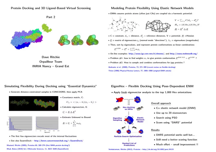
EigenHex – Flexible Docking Using Pose-Dependent ENM

• Apply fresh eigenvector analysis to the top 1,000 Hex orientations

Overall approach

• Cα elastic network model (ENM)
• Use up to 20 eivenvectors
• Search using PSO
• Score using “DARS” potential

Results

• DARS potential works well but...
• Still need a better scoring function
• Much effort – small improvement !!

Venkatraman, Ritchie (2012), Proteins – http://dx.doi.org/10.1002/prot.24115

RosettaDock – Flexible Refinement by Side Chain Re-Packing

• Given a rigid body starting pose, repeat 50 times:
• REMOVE and RE-BUILD side chains; apply local rigid-body minimisation
• apply Monte-Carlo accept/reject
• Successful for several CAPRI targets; also works well for 50% of Docking Benchmark v2

Gray (2006) Current Opinion in Structural Biology, 16, 183–193

Haddock – “Highly Ambiguous Data-Driven Docking”

• Flexible refinement using CNS with ambiguous interaction restraints (AIRs)
• Use of “active” and “passive” residues ensures active residues at interface
• E.g. residue i of protein A:

deff

iAB =

NiA

miA=1

NresB

k=1

NkB

nkB=1

• 1

d6

miA,nkB

−1/6

• V. good CAPRI results
• Restraints from (e.g.):

SAXS mutagenesis mass spectroscopy NMR (RDC, CSP)

van Dijk et al. (2005) FEBS J, 272, 293–312 van Dijk et al. (2005) Proteins, 60, 232–238

Knowledge-Based Protein Docking: CAPRI Target 40 (2009) – API-A/Trypsin

• We searched SCOPPI and 3DID for similar domain interactions to the target
• This helped to identify two key inhibitory loops on API-A around L87 and K145
• Performing focused Hex + MD refinement gave a total of 9 “acceptable” solutions

The KBDOCK Database and Web Server

• Content: 2,721 non-redundant hetero DDIs involving 1,029 PFAM domain families
• For each PFAM family, all DDIs are superposed and spatially clustered

http://kbdock.loria.fr/

• Aim: to provide PFAM family-level structural templates for knowledge-based docking

KBDOCK – Analysis of PFAM Domain Family Binding Sites

• Nearly 70% of PFAM domain families have just one binding site
• Very few domains have more than two or three binding sites
• This supports the notion that protein binding sites are often re-used...

KBDOCK – Template-Based Protein Docking Results

• The Protein Docking Benchmark 4.0 contains 176 protein-protein complexes
• We selected 73 single-domain complexes
• A “Full-Homology” (FH) template matches both target domains
• A “Semi-Homology” (SH) template matches just one target domain

Target Total FH Two SH One SH Zero class targets templates templates template templates Without date filtering Enzyme 36 24 / 24 (3 + 1) / 5 3 / 5 2 Other 37 21 / 21 (0 + 0) / 3 5 / 11 2 With date filtering Enzyme 36 13 / 13 (2 + 1) / 5 7 / 11 7 Other 37 13 / 13 (0 + 0) / 1 8 / 15 8

• If a FH template exists, it is almost always correct
• Even if there is no FH template, SH templates can still provide useful information

Ghoorah et al. (2011), Bioinformatics, 27, 2820–2827

Assembling Multi-Component Protein Complexes

• Multi-component assembly is a highly combinatorial problem
• How to generate and score candidate orientations efficiently?
• Here, we use Minimum Weight Spanning Trees (MSTs), (Inbar et al., 2003)
• ... with an ant colony particle swarm optimisation (PSO) search algorithm

Inbar et al. (2003), Bioinformatics, 2003, i158–i168

Minimum Energy Spanning Trees

• Here, we have N = 5 proteins and K = N(N-1)/2 = 10 “edges”
• Each edge should consider many (e.g. P = 100) docking solution
• Naive enumeration would give P N(N−1)/2 possible combination
• A spanning tree visits each node just once...
• ... there are only P N−1N N−2 distinct spanning trees
• ... and when N < P, we get P N−1N N−2 << P N(N−1)/2
• Strategy: search for the minimum energy spanning tree ...
• Getting technical: this is an “edge-weighted K-cardinality” problem...

Multi-Component Docking using Ant-Colony Optimisation

Ant colonly optimisation is based

• n the behaviour of real ants

When an ant finds food, it leaves a trail of pheromones Other ants follow strong pheromones trails to reach the food quickly

• Here, we use 10 ants in parallel for 1,000 iterations...
• Each ant is asigned to a randomly generated spanning tree
• It must detect and score steric clashes, and update its trail
• It then makes a new spanning tree using the latest pheromone trails...

MDOCK – Multi-Component Docking Results

• There are not many multi-component examples in the PDB
• Therefore, several ‘targets” were made from the same complex...
• 1VCB = von Hippel-Lindau ElonginC-ElonginB tumor suppressor protein
• 1IKN = Transcription factor I-kappa-B-alpha / NF-kappa-B
• 1K8K = Bovine actin polymerisation initiation complex Arp2 / Arp3

Target Chains Time (min) Rank RMSD (˚ A) Best RMSD (˚ A) 1VCB A,B,C 43.8 1 0.58 0.58 1IKN A,C,D 77.3 1 9.17 0.88 1K8K A,B,D,E 123.5 1 4.96 2.19 1K8K A,B,D,E,F 168.6 2 9.48 2.99 1K8K A,B,D,E,F,G 194.1 15 4.63 3.53 1K8K A,B,C,D,E,F,G 366.9 – – 10.21

• Mostly good results, but why did we miss one?
• However, it would be very expensive to apply this algorithm to blind docking ...

Venkatraman, Ritchie (2012), in press.

The Inside of a Cell is Highly Crowded

• This image shows a model of the cytoplasm in E. Coli
• Can we use docking algorithms to predict the protein-protein interactions ?

McGuffee, Elcock (2009), PLoS Comp Biol, 6, e1000694

Large-Scale Cross-Docking Has Only Recently Become Feasible

• Wass et al. used Hex to cross-dock 56 true protein pairs with 922 non-redundant “decoys”
• For each pair, they plotted the profile of the best 20,000 docking scores...

(negative scores are good; red/blue = correct PPI; red/cyan = incorrect interactions)

• 48/56 true PPIs have significantly (statistically) higher energies than background false pairs
• Only 8/56 true PPIs have indistinguishable profiles to the non-binders
• NB. this experiment is detecting energy funnels, not necessarily the correct docking pose

Wass et al. (2011) Molecular Systems Biology, 7, article 469

IMP – Integrative Modeling Platform

• Python-based system for integrative multi-component modeling – http://salilab.org/imp/
• Combines structural data from: cryoEM (mainly), X-Ray, NMR, SAXS, Modeller, ...

... with interaction data from BioGRID – http://thebiogrid.org/

• The overall approach is to maximise a multi-term objective function:

F =

i αi + i<j βij

αi are single-body terms (e.g. goodness of fit in a density map, protrusion penalty) βij are two-body terms (e.g. the docking score for two proteins in contact)

• But it is a *highly* combinatorial search space, with missing/incomplete data...

Russel et al. (2012) PLoS Biology, 10, e1001244 Lasker et al. (2009) J Molecular Biology, 388, 180–194

Putting The Pieces Together – The Nuclear Pore Complex

• The NPC has some 650 components – raw data at http://salilab.org/npc
• It required an immense multi-disciplinary effort to build this model ...
• See Dreyfuss et al. for an interesting computational validation of the model

Alber et al. Nature (2007) 450, 683–694 and 695–701 Dreyfuss et al. Proteins (2012) – http://dx.doi.org/10.1002/prot.24092

But What About the Virtual Screening ? Protein-Drug Interaction Resources

“The availability of interaction data between small molecule drugs and protein targets has increased sub- stantially in recent years... We assembled a total of 4,767 unique interactions between 802 drugs and 480 targets, which means that on average every drug interacts with at least 6 targets...” Mestres et al., (2009).

• STITCH – Search Tool for Interactions of Chemicals – http://stitch.embl.de
• 68,000 chemicals (including 2,200 drugs) linked to 1.5 million genes
• ChEMBL – database of drug-like bioactive molecules – https://www.ebi.ac.uk/chembldb/
• Binding & toxicity data for 1.1 million compounds and 5,200 protein targets

Mestres et al. (2009) Molecular BioSystems, 5, 1051–1057 Kuhn et al. (2008) Nucleic Acids Research, 36, D684–D688 (STITCH) Gaulton et al. (2012) Nucleic Acids Research, 40, D1100–D1107 (ChEMBL)

A Growing Interest in Drug Promiscuity and Drug Repositioning

• Approx 90% of new drugs fail to reach market – often due to toxicity or lack of efficacy

toxicity – e.g. from unwanted off-target interactions lack of efficacy – e.g. from robustness of biological network

• Example – PROMISCUOUS – http://bioinformatics.charite.de/promiscuous/

“network-based drug repositioning” – 25K drugs, 21K drug-protein, 104K PPIs

von Eichborn et al. (2011) Nucleic Acids Research, 39, D1060–D1066 (PROMISCUOUS) Kuhn et al. (2011) Molecular Systems Biology, 6, 343 (SIDER)

Atomic Resolution Studies of Hetero PPIs and Inhibitors

• TIMBAL – http://www-cryst.bioc.cam.ac.uk/timbal/ – 27 structures, 104 small molecules
• 2P2I (= PPI inhibition) – http://2p2idb.cnrs-mrs.fr/ – 17 PPIs, 56 small molecules
• The ligands generally have high MW and are hydrophobic
• The PPIs have few/no small interface pockets; small conformational changes on binding
• See also Dr. PIAS – http://www.drpias.net/ – SVM-based prediction of druggable PPIs

Higueruerlo et al. (2009) Chemical Biology Drug Design, 74, 457–467 (TIMBAL) Borgeas et al. (2010) PLoS One, 4, e9598 (2P2I) Sugaya, Furuya (2011) BMC Bioinformatics, 12, 50 (Dr. PIAS)

A Gaussian Representation of Molecular Shape

• Represent each atom in a molecule as a 3D Gaussian density function:

ρi(r) = βe−γr2/σ2

i

and choose β, γ such that:

• ρi(r)dx = 4

3πσ3 i

where σi = van der Waals radius of atom i

• Represent the “density” of a molecule as a sum of N atomic densities:

ρ =

i<N ρi − i<j<N ρiρj + i<j<k<N ρiρjρk − ...

= 1 − ΠN−1

i=0 (1 − ρi)

• Some examples:

Grant et al. (1996) J Computational Chemistry, 17, 1653–1666

Gaussian Overlap Volumes and Tanimoto Scores

• The overlap volume between two atomic Gaussians is just another Gaussian:

Vij =

• ρiρjdx

= βiβj

• π

αi+αj

3/2e

−(

αiαj αi+αj )R2 ij

where Rij is distance between the atom centres, and αi = γ/σ2

i

• Hence the overlap volume between two molecules can also be calculated easily...

... and normalised to give a Tanimoto-like similarity score (with range 0 < SAB ≤ 1.0 ): VAB =

• ρAρBdx

SAB =

VAB VAA+VBB−VAB

... and this is easy to optimise:

δVij δx = −2( αiαj αi+αj)(xi − xj)Vij

etc.

Haigh, Pickup (2005), J Chemical Information & Modeling, 45, 673–684

ROCS – “Rapid Overlay of Chemical Structures”

• ROCS is a commercial implementaton of the Gaussian representation of Grant at al.
• ROCS initially uses “steric multipoles” to align molecules with the Cartesian axes

Mpq =

• pqρdx, where each p and q stands for x, y, or z

Diagonalising M is equivalent to finding the principal ellipsoidal axes...

• ROCS then maximises the Gaussian overlap starting from 4 different orientations (axis flips)
• Recently, “FASTROCS” (GPU-based version) – up to 106 superpositions/second !!

http://www.eyesopen.com/rocs/ Haque, Pande (2009), J Computational Chemistry, 31, 117–132 (open source GPU version)

ParaSurf – SH Surfaces & Properties from Semi-Empirical QM

• From MOPAC or VAMP calculate:
• Density contours of 2 × 10−4e/˚

A

3 ( ∼ SAS)

• Key local properties: MEP, IEL, EAL, αL
• Encode as SH expansions to L=15:

f(θ, φ) = L

l=0

l

m=−l flmylm(θ, φ)

Lin, Clark (2005), J Chemical Information & Modeling, 45, 1010–1016 Clark (2004), J Molecular Graphics, 22, 519–525

ParaFit – High Throughput SH Surface & Property Matching

Distance: D =

• (rA(θ, φ) − rB(θ, φ)′)2dΩ

(in units of area) Orthogonality: D = |a|2 + |b|2 − 2a.b′ Rotation: b′

lm =

• m′

R(l)

mm′(α, β, γ)blm′

Hodgkin: S = 2a.b′/(|a|2 + |b|2) Carbo: S = a.b′/(|a|.|b|) Tanimoto: S = a.b′/(|a|2 + |b|2 − a.b′) Multi-property: S = pSshape + qSMEP + rSIEL + sSEAL + tSαL

Perez-Nueno et al. (2010), Molecular Informatics, 30, 151–159

Brute-Force Spherical Harmonic Surface Superpositions

• Generate 22,500 Euler rotations from icosahedral tesselation of sphere
• Refine with 16 × 16 × 16 grid of 1 degree steps (gives about 50 molecules / second)
• Can also pre-process a set of molecules by aligning them to the principal axes

z x

• Pre-aligned “canonical” orientations of similar molecules often overlay very well ...

Clustering the Odour Dataset using 2D SH Surface Shapes

(Takane et al. (2004) Org. Biomol. Chem. 2 3250–3255)

• Seven classes: bitter, ambergris, camphoraceous, rose, jasmine, muguet, musk
• Following Takene et al., we clustered into 10 group using ParaSurf & Parafit:

unix% PS mopac run unix% PS parasurf run unix% parafit -matrix -dif odour data.dif * p.sdf unix% dif2jpg -n 10 -d odour data.dif unix% eog odour data.jpg

Visualising The Odour Dataset Clustering Results

Clustering Superposed Pairs Clustering Canonical Orientations

Mavridis et al. (2007), J Chemical Information & Modeling, 45, 1787–1796

Promiscuous Protein Targets Seem to be Rather Common

• Example: ALR2 is know to bind at least 5 different ligand scaffold families...
• Several other promiscuous targets in the literature:
• the α1β1 and α2β1 integrins,
• factor H, LRP6, PPAR-γ, LXR-β,
• ACHE, P38, FXA, VEGFR2, PXR,
• β-secretase, thrombin, CDK2,
• LAIR-1, LAIR-2, LTBLP-2, NS2B-NS3.
• For ligand-based virtual screening, these examples suggest:
• cluster the 3D shapes of any known ligands before performing VS ...
• compare shape-based VS performance with and without clustering ...
• ... any large differences could suggest a promiscuous (multi-site?) substrate.

P´ erez-Nueno, Ritchie (2011). Expert Opinion on Drug Discovery, 7, 1–17

Ligand-Based VS (LBVS) Principals

• LBVS aims to find new actives by similarity to one or more existing actives
• Usually LBVS has two phases – retrospective (i.e. “training mode”), and prospective
• Main purpose of retrospective VS is to find the best algorithm + query (molecule/conformation)
• Prerequisites: some know actives + a good set of decoys (similar mol wt, chemistry)
• Historically, enrichment plots have been popular for analysing ranked lists of VS results
• Disadvantages:
• enrichment plots (or enrichment factors) depend on the no. of actives
• it is difficult to compare different enrichment plots

Receiver-Operator-Characteristic (ROC) Plots

• ROC plots show the ability of a classifier to distinguish postive and negative instances
• A ROC plot shows the true positive rate (TPR) against the false positive rate (FPR)
• Suppose 10 positive and 10 negative instances have been scored by a classifier...

Score Class Npos Nneg TPR FPR

• ---- ----- ---
• 0.90

pos 1 0.1 0.0 0.80 pos 2 0.2 0.0 0.70 neg 2 1 0.2 0.1 0.60 pos 3 1 0.3 0.1 0.55 pos 4 1 0.4 0.1 0.54 pos 5 1 0.5 0.1 0.53 neg 5 2 0.5 0.2 0.52 neg 5 3 0.5 0.3 0.51 pos 6 3 0.6 0.3 0.50 neg 6 4 0.6 0.4 0.40 pos 7 4 0.7 0.4 0.39 neg 7 5 0.7 0.5 0.38 pos 8 5 0.8 0.5 0.37 neg 8 6 0.8 0.6 0.36 neg 8 7 0.8 0.7 0.35 neg 8 8 0.8 0.8 0.34 pos 9 8 0.9 0.8 0.33 neg 9 9 0.9 0.9 0.32 pos 10 9 1.0 0.9 0.31 neg 10 10 1.0 1.0

0.0 0.2 0.4 0.6 0.8 1.0 0.0 0.2 0.4 0.6 0.8 1.0 ROC Plot

FPR TPR

• The area under the curve (AUC) gives a good overall measure of classifier performance
• A random classifier gives a diagonal line: TPR=FPR (AUC=0.5)
• A perfect classifier gives TPR=1.0 for all FPR (AUC=1.0)

Fawcett (2006) Patttern Recognition Letters 27, 861–874; en.wikipedia.org/wiki/Receiver operating characteristic

Several Other Common VS Quality Measures

• Suppose there are n actives in a total of N molecules, and the scoring function

is used to produce a ranked list of molecules: i = 1, 2, 3, ...N.

• Often we are most interested in the quality of the top (e.g. top 1%) of the ranked list
• Enrichment Factor:

EFx% = na/Nx%

n/N

• ROC AUC:

AUC = 1

n

n

i=1(1 − fi)

• ROC AUCx% :

AUCx% = calculate graphically

• Balanced ROC:

BAROC = 1

n

n

i=1 e−αfi

• Sum of Logs of Rank:

SLR = − n

i=1 log

ri

N

• Normalised SLR:

NSLR = n

i=1 log

ri

N

• / n

i=1 log

i

N

• (here, the top x% of the list contains Nx% molecules and na actives, ri is the

rank of the ith active, and fi is the fraction of inactives ranked higher than i)

• Which is best? Debatable! These days, ROC AUC, AUC5%, AUC10% are quite popular...

Venkatraman et al. (2010), J Chemical Information & Modeling, 50, 2079–2093

Comparing Ligand-Based Virtual Screening Methods

• We calculated aggregate ROC plots to compare several VS methods on the “DUD” dataset
• DUD = Directory of Useful Decoys – http://dud.docking.org/ – 40 targets, 100K decoys
• 2D methods = Babel, Daylight, MACCS, MCI, Molprint2D
• 3D methods = Parafit, ROCS, SHAEP, USR, Eshape3D
• The fingerprint methods perform remarkably well (!)
• Suggests need to improve 3D methods – better query conformations ? shape clustering ?

Venkatraman et al. (2010), J Chemical Information & Modeling, 50, 2079–2093

Conclusions

• Modeling flexibility during docking is still a major challenge
• Cross-docking can detect protein-protein partners remarkably often
• Knowledge-based protein docking is becoming increasingly useful
• Most Pfam families have just one binding site – often re-used
• Several proteins bind multiple ligand families – promiscuous targets
• Fast 3D virtual screening algorithms are becoming available
• All-vs-all 3D protein docking and ligand shape-matching now feasible ?
• Choosing a good query conformation still a challenge in ligand-based VS

Acknowledgments Anisah Ghoorah Matthieu Chavent Diana Mustard Lazaros Mavridis Violeta P´ erez-Nueno Vishwesh Venkatraman BBSRC, EPSRC, ANR Software & Papers: http://hex.loria.fr/ HexServer: http://hexserver.loria.fr/