protein docking and 3d ligand based virtual screening
play

Protein Docking and 3D Ligand-Based Virtual Screening Schedule - PowerPoint PPT Presentation

Protein Docking and 3D Ligand-Based Virtual Screening Schedule Lecture 1 Rigid Body Protein Docking Part 1 Introduction / Motivation Protein Docking and the CAPRI Blind Docking Experiment The Hex Spherical Polar Fourier


  1. Protein Docking and 3D Ligand-Based Virtual Screening Schedule • Lecture 1 – Rigid Body Protein Docking Part 1 • Introduction / Motivation • Protein Docking and the CAPRI Blind Docking Experiment • The “Hex” Spherical Polar Fourier Correlation Algorithm • Ultra-Fast Docking Using Graphics Processors (+ some GPU programming) • Lecture 2 – New Developments in Protein Docking and Virtual Screening • Simulating Protein Flexibility During Docking • Data-Driven and Knowledge-Based Docking • Multi-Component Assembly and Cross-Docking • Shape-Based Virtual Screening – ROCS, ParaSurf, ParaFit Dave Ritchie • Lecture 3 – Spherical Harmonic Virtual Screening Orpailleur Team • Case Study – HIV Entry Inhibitors for the CXCR4 and CCR5 Receptors INRIA Nancy – Grand Est • Recent Work – Detecting Polypharmacology Using Gaussian Ensemble Screening 
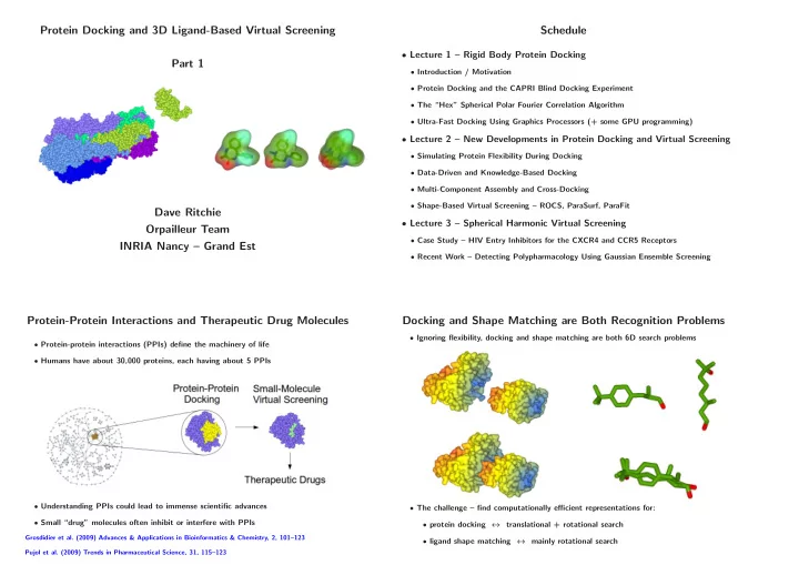
Protein-Protein Interactions and Therapeutic Drug Molecules Docking and Shape Matching are Both Recognition Problems • Ignoring flexibility, docking and shape matching are both 6D search problems • Protein-protein interactions (PPIs) define the machinery of life • Humans have about 30,000 proteins, each having about 5 PPIs • Understanding PPIs could lead to immense scientific advances • The challenge – find computationally efficient representations for: • Small “drug” molecules often inhibit or interfere with PPIs • protein docking ↔ translational + rotational search Grosdidier et al. (2009) Advances & Applications in Bioinformatics & Chemistry, 2, 101–123 • ligand shape matching ↔ mainly rotational search Pujol et al. (2009) Trends in Pharmaceutical Science, 31, 115–123

  2. Protein-Protein Interaction Challenges Protein-Protein Interaction Resources • Can we predict the interactions within a proteome – i.e. predict the interactome ? • STRING – Search Tool for Retrieval of Interacting Genes – http://string.embl.de • 12 million known PPIs; 44 million predicted • 3DID – 3D Interacting Domains – http://3did.irbbarcelona.org • 160,000 3D domain-domain interactions (DDIs) • For each interaction, can we predict the interface surfaces and the 3D complex ? • For each protein can we predict its ligand binding sites ? Stein et al. (2010) Nucleic Acids Research, 33, D413–D417 (3DID) Wass, David, Sternberg (2011) Current Opinion in Structural Biology, 21, 382–390 Szklarzyk et al. (2011) Nucleic Acids Research, 39, D561–D568 (STRING) What is Protein Docking and Why is Docking Difficult ? The CAPRI Blind Docking Experiment • Protein docking = predicting protein interactions at the molecular level • Critical Assessment of PRedicted Interactions – http://www.ebi.ac.uk/msd-srv/capri/ • Given the unbound structure, particiants have to predict the unpublished 3D complex T8 = nidogen/laminin T9 = LiCT dimer T10 = TEV trimer T11-12 = cohesin/dockerin T13 = Fab/SAG1 T14 = PP1 δ /MYPT1 • If proteins are rigid = > six-dimensional search space T15 = colicin/ImmD • But proteins are flexible = > multi-dimensional space! T18 = Xylanase/TAXI • Modeling protein-protein interactions accurately is difficult! T19 = Fab/bovine prion Halperin et al. (2002), Proteins, 47, 409–443 Janin (2005) Proteins, 60, 170–175 Ritchie (2008), Current Protein & Peptide Science, 9, 1–15

  3. CAPRI Target T6 Was A Relatively Easy Target CAPRI Target T27 Was A Surprisingly Difficult Target • Amylase / AMD9 showed little difference between unbound & bound conformations • Arf6 GTPase / LZ2 Leucine zipper was difficult for most CAPRI predictors • It also had a classic binding mode, with antibody loops blocking the enzyme active site • Best = superposition • Circles show LZ2 centres: blue = high quality green = medium quality cyan = acceptable qlauity yellow = wrong • Several CAPRI predictors made “high accuracy” models (Ligand RMSD ≤ 1˚ A) Janin (2010) Molecular BioSystems, 6, 2362–2351 ICM – Multi-Start Pseudo-Brownian Monte-Carlo Energy Minimisation PatchDock – Docking by Geometric Hashing • Use “MS” program to calculate mesh surfaces for each protein • Start by sticking “pins” in protein surfaces at 15˚ A intervals • Divide the mesh into convex “caps”, concave “pits”, and flat “belts” • Find minimum energy for each pair of starting pins (6 rotations each): E = E HV W + E CV W + 2 . 16 E el + 2 . 53 E hb + 4 . 35 E hp + 0 . 20 E solv • For docking, match pairs of concave ↔ convex, and flat ↔ any ... ... then test for interpenetrations (steric clashes) between rest of surfaces • The method is fast (minutes/seconds), and gave good results in CAPRI Duhovny et al. (2002), LNCS 2452, 185–200 • ICM achieved the best overall results in the first few rounds of CAPRI ... Schneidman-Duhovny et al. (2005), Nucleaic Acids Research, 33, W363–W367 Fern´ andez-Recio, Abagyan (2004), J Mol Biol, 335, 843–865 Connolly (1983), J Applied Crystallography, 16, 548–558

  4. Predicting Protein-Protein Binding Sites Protein Docking Using Fast Fourier Transforms • Many algorithms / servers are available for predicting protein binding sites • Conventional approaches digitise proteins into 3D Cartesian grids... • For recent review, see: Fern´ andez-Recio (2011), WIREs Comp Mol Sci 1, 680–698 • Many docking algorithms often show clusters of preferred orientations – docking “funnels” • ...and use FFTs to calculated TRANSLATIONAL correlations: C [∆ x, ∆ y, ∆ z ] = � x,y,z A [ x, y, z ] × B [ x + ∆ x, y + ∆ y, z + ∆ z ] • BUT for docking, have to REPEAT for many rotations – EXPENSIVE! • Lensink & Wodak proposed that docking methods are the best predictors of binding sites • Conventional grid-based FFT docking = SEVERAL CPU-HOURS Fern´ andez-Recio, Abagyan (2004), J Molecular Biology, 335, 843–865 Lensink, Wodak (2010), Proteins, 78, 3085–3095 Katchalski-Katzir et al. (1992) PNAS, 89 2195–2199 Knowledge-Based Protein-Protein Docking Potentials DARS Finds More Hits Than ZDOCK and Shape-Only Docking • Several groups have developed “statistical” potentials based on “inverse Boltzmann” models • Comparing the no. of “hits” for 33 enzyme-inhibitor complexes... • Example – PIPER + DARS – “Decoys As Reference State” – http://structure.bu.edu/ • Define 18 atom types (based on ACP potential): N, CA, C, O, GC, CB, KN, KC, DO, ... IJ /P ref • Define interaction energy: E IJ = − RT ln( P nat IJ ) • P nat = probability of contact between atom I and J in a native complex IJ (use 20 CAPRI complexes as examples containing native complexes) • P ref = probability of contact between atom I and J in a reference state IJ (use PIPER Cartesian FFT to generate 20,000 “decoy complexes” for each native) • Count each type of contact (6˚ A threshold) to make the probabilities • This gives a matrix of 18 x 18 atomic interaction energies • Clever trick: diagonalise the matrix to get the first 4 or 6 leading terms... (allows PIPER to use 4 or 6 FFTs instead of 18) • PIPER + DARS is one of the best approaches in CAPRI... • DARS potential = red; ZDOCK (ACP) = green; shape-only = blue Kozakov et al. (2006) Proteins, 65, 392–406 Kozakov et al. (2006) Proteins, 65, 392–406

  5. Protein Docking Using Polar Fourier Correlations Some Theory – The Spherical Harmonics • The spherical harmonics (SHs) are examples of classical “special functions” • Rigid body docking can be considered as a largely ROTATIONAL problem • Spherical polar coordinates: r = ( r, θ, φ ) • This means we should use ANGULAR coordinate systems z z r=(r, θ,φ) θ α B r y β B φ y x γ B x z R • The spherical harmonics are products of Legendre polynomials and circular functions: β A • Real SHs: y lm ( θ, φ ) = P lm ( θ ) cos mφ + P lm ( θ ) sin mφ y γ A Y lm ( θ, φ ) = P lm ( θ ) e imφ • Complex SHs: x • Orthogonal: � y lm y kj dΩ = � Y lm Y kj dΩ = δ lk δ mj j R ( l ) y lm ( θ ′ , φ ′ ) = � • Rotation: jm ( α, β, γ ) y lj ( θ, φ ) • With FIVE rotations, we should get a good speed-up? Spherical Harmonic Molecular Surfaces Docking Needs a 3D “Spherical Polar Fourier” Representation • Use SHs as orthogonal shape “building blocks”: • Need to introduce special orthonormal Laguerre-Gaussian radial functions, R nl ( r ) • Encode distance from origin as SH series to order L: • R nl ( r ) = N ( q ) nl e − ρ/ 2 ρ l/ 2 L ( l +1 / 2) ρ = r 2 /q, n − l − 1 ( ρ ); q = 20 . • r ( θ, φ ) = � L � l m = − l a lm y lm ( θ, φ ) l =0 R 15 , 0 ( r ) Solvent Accessible Surface Surface Skin 30 • Reals SHs: y lm ( θ, φ ) R 20 , 0 ( r ) Molecular Surface Sampling 30 Spheres • Coefficients: a lm R 25 , 0 ( r ) Surface Protein Interior 30 • Solve the coefficients by numerical integration Normals R 30 , 0 ( r ) 30 • Normally, L=6 is sufficient for good overlays � � 1; r ∈ surface skin 1; r ∈ protein ato • Surface Skin: σ ( r ) = Interior: τ ( r ) = 0; otherwise 0; otherwise σ ( r ) = � N � n − 1 � l m = − l a σ • Parametrise as: nlm R nl ( r ) y lm ( θ, φ ) n =1 l =0 n ′ l ′ T ( | m | ) nlm = � N • TRANSLATIONS: a σ ′′ nl,n ′ l ′ ( R ) a σ n ′ l ′ m Ritchie and Kemp (1999) J Computational Chemistry, 20, 383–395 Ritchie (2005) J Applied Crystallography, 38, 808–818 (for translation formulae)

Download Presentation
Download Policy: The content available on the website is offered to you 'AS IS' for your personal information and use only. It cannot be commercialized, licensed, or distributed on other websites without prior consent from the author. To download a presentation, simply click this link. If you encounter any difficulties during the download process, it's possible that the publisher has removed the file from their server.

Recommend


More recommend