Projects (upcoming) Assess Portfolio Machine Learning for Trading - - PowerPoint PPT Presentation

Machine Learning for Trading Software Platform Introduction & Installation

Projects (upcoming)

• Assess Portfolio
• Assess Learners & Defeat Learners
• Market Simulator

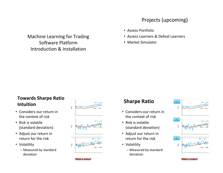
Towards Sharpe Ratio Intuition

• Considers our return in

the context of risk

• Risk is volatile

(standard deviation)

• Adjust our return in

return for the risk

• Volatility

– Measured by standard deviation

Sharpe Ratio

• Considers our return in

the context of risk

• Risk is volatile

(standard deviation)

• Adjust our return in

return for the risk

• Volatility

– Measured by standard deviation

1 2 3

Sharpe Ratio

• 1. Higher Returns is Better
• 2. Less Volatility/Less Risk

is Better

• 3. Not Enough Information

– Returns: ABC > XYZ – Volatility ABC > XYZ – ABC is higher returns, but more risk

1 2 3

Sharpe Ratio

• Adjusts the

– return for risk

• A quantitative way to assess a portfolio

– 1. ABC is better because it has the same volatility but higher returns – 2. same returns but XYZ has lower risk so XYZ is better – 3. A quantity such as the Sharpe Ratio may give you a number to determine which is better

• Sharpe ratio also considers (comparative)

– Risk free rate of returns

• Example Bank account or treasure note

– Lately risk free return is 0, bank interest rate is 0, or close to 0 – Caveat: When computing Sharpe Ratio need to be careful of the risk free returns rate:

• Annual, weekly, daily

Intuition: Which Formula is Best?

Consider Parameters to include in formula:

• Rp : Portfolio Return
• Rf : Risk Free Rate of Return
• σp : Standard Deviation of Portfolio Return

a) Rp – Rf + σp b) Rf / Rf - σp c) (Rp – Rf) / σp

General Form of the Sharpe Ratio

Heuristics Sharpe Ratio

• Sharpe Ratio Answers: Is the

portfolio return due to intelligent investment decisions or the result

• f excessive risk taken by the

investor?

• The greater a portfolio’s Sharpe

ratio:

• The better its risk-adjusted

performance has been.

• A negative Sharpe ratio indicates that

a risk-less asset (risk free) would perform better than the portfolio (return) being analyzed.”

Computing Sharpe Ratio

• Expected return : Can use mean() of daily returns

(accessible via yahoo finance).

• StD() of daily returns.
• StD() of the Return of the Risk Free Rate

– Standard deviation of a constant is 0 (can remove).

• What is the risk free rate?

– LIBOR (London Inter Bank Offer Rate) – Interest Rate: 3 months Treasury Bill (Standard) – 0%! Short Cut. – If you use daily returns, then the risk free rate needs to be at the same sampling rate:

• So if you are referencing an annual rate then you will need to convert it

to a daily risk free rate.

Risk Free Rate

• If you have annual rate and want Effective

Daily Rate compounded daily.

• Caveat: Compound interest is not linear with

time. Example: 2.5% Annual Return - Going to effective daily return – 242 trading days in a year.

=POWER(1+0.025,1/242)-1

1+ Annualized Return

Nth

−1 1+0.025

242

−1

• Sharpe Ratio itself is an annual measure, so if

we are sampling at a different rate e.g. daily, need an adjustment factor to convert it to the correct period

– SRannualized= k * SR

Sample Rate K (convert to annual) Daily Weekly Monthly

SR =

Computing SR Summary

• 2 things to consider when computing Sharpe

Ratio:

– 1) Convert Risk Free Rate to same period as expected return period. – 2) Convert SR to annual SR. (using adjustment factor k).

Quiz: What is the Sharpe Ratio?

• 60 Days of Data
• BPS – Basis points are tenths of percentages.
• Average Daily Return = 10 bps = 0.001
• Daily Risk Free Rate = 2 bps = 0.0002
• Standard Deviation Daily Return = 10 bps = 0.001

SR = SQRT ( Period ) * mean (Rportfolio- RRiskFree)

• Std( Daily Return)

SR = SQRT ( Period ) * (10-2)

• 10

Quiz: What is the Sharpe Ratio?

• 60 Days of Data
• BPS – Basis points are tenths of percentages.
• Average Daily Return = 10 bps = 0.001
• Daily Risk Free Rate = 2 bps = 0.0002
• Standard Deviation Daily Return = 10 bps = 0.001

SR = SQRT ( Period ) * mean (Rportfolio- RRiskFree)

• Std( Daily Return)

SR = SQRT ( Period ) * (10-2)

• 10

Project Demo

• Compute port_val and statistics…

Get the Daily Total Value of the Portfolio

• Step 1: Prices Data Frame index by dates

– prices is a frame.

• Step 2: Normalize by First Row

– normed = prices/prices[0]

• Step 3: Multiply by allocation (a vector)

– allocated = normed * allocs

• Step 4: Position values = worth each day

– pos_vals = allocated * start_val

• Step 5: Daily Total Value of Portfolio

– port_vals = pos_vals.sum(axis = 1)

prices normed allocated pos_vals port_vals

Given: Given: start_val start_val = $1,000,000 = $1,000,000 start_date start_date = 2011-01-01 = 2011-01-01 end_date end_date = 2011-12-31 = 2011-12-31 symbols =[‘SPY’,’XOM’, symbols =[‘SPY’,’XOM’, ’GOOG’, ‘GLD’] ’GOOG’, ‘GLD’] allocs = [0.4,0.4,0.1,0.1] allocs = [0.4,0.4,0.1,0.1]

prices/prices[0] normed/allocs allocated * start_val pos_vals.sum( axis = 1 )

port_vals = get_portfolio_value( prices, allocs, start_val)

Compute Statistics

• Average Daily Return

– Intuition :

• Today/Yesterday - 1
• Remove 1st row since now it is all 0s

– Excel a cell G10 = E10/E9-1

• E10 = current’s row adjusted close
• E09 = previous day’s adjusted close

– Pandas:

• daily_rets = port_val / port_val.shift(X) - 1
• # what is X?
• Cumulative from beginning to end

– >= period than daily return.

• Average and Standard Deviation of the

Daily Return .mean(), .std()

• Sharpe Ratio (Annual)

Given: Given: 1) 1) port_vals port_vals: portfolio : portfolio daily return values daily return values 2) 2) rfr rfr: risk free rate : risk free rate 3) sample_frequency: Sample : Sample Frequency Frequency – Example, Example, daily 252 in a year. daily 252 in a year.

cr, adr, sddr, sr = get_portfolio_stats( port_val, risk_free_rate, sample_frequency)

Optimization

• What is an optimizer?
• 1. Find minimum values of functions
• Example: f(x) = x2 + x3 + … + 1
• 2. Find parameters from data
• Enables: building parameterized models based on data
• How: polynomial fit to data
• 3. Find (refine) allocation of stocks in a portfolio
• What percentage should be allocated to each stock to

maximize the portfolio return (part of the project).

Find Minima of a Function

• How to use an optimizer:

1) Provide a function to minimize:

• Example: f(x) = x2 + 0.5

2) Provide an initial guess:

• Example = 5 (generated by a randomizer)

3) Call the optimizer with the parameters above

Example: Minimization

1) Function provided:

– f(x) = (x – 1.5)2 + 0.5

2) Provide an initial guess: 3.0 3) Call Optimizer with parameters defined above.

– One method:

• Gradient descend to narrow in on

the solution.

• Experiment with other methods.
• Next: Look at Code (provided):

– pdf-code-finance/001-minimizer.py

http://www.wolframalpha.com/ min( x- 1.5)^2 + 0.5 ) f(x) : Y = (X - 1.5)**2 + 0.5 # parabola at X = 1.5 Y = 0.5 min_result = spo.minimize(f, Xguess, method='SLSQP', options = {'disp':True})

Exercise: Minimization

1) Function provided:

– f(x) = (x1 )2 + (x2 )2

2) Provide an initial guess: [1,1] 3) Call Optimizer with parameters defined above.

– One method:

• Gradient descend to narrow in on

the solution.

• Experiment with other methods.
• Code Snippets:

http://www.wolframalpha.com/ min(X1^2 + X2^2) x1, x2 = params Z = x1**2 + x2**2 Xguess = [1,1] min_result = spo.minimize(f, Xguess, method='SLSQP', options = {'disp':True})

• ptimize1D2.py

Exercise: Minimization

1) Function provided:

– f(x) = (x1 )2 + (x2 )2

2) Provide an initial guess: [1,1] 3) Call Optimizer with parameters defined above.

– One method:

• Gradient descend to narrow in on

the solution.

• Experiment with other methods.
• Code Snippets:

http://www.wolframalpha.com/ min(X1^2 + X2^2) x1, x2 = params Z = x1**2 + x2**2 Xguess = [1,1] min_result = spo.minimize(f, Xguess, method='SLSQP', options = {'disp':True})

• ptimize1D2.py

Exercise

#min (X1+0.5)^2 + (X2-0.25)^2+sin(3X1)+sin(5X2)

Which functions are challenging to solve (for the minimizer)?

• A
• B
• C
• D

Which functions are challenging to solve (for the minimizer)?

• A – flat areas don’t have a gradient.
• B - convex problems
• C – several global minima
• D – discontinuity (and a flat area).
• Convex functions are guaranteed to find a

minima (only one).

• But – other algorithms for specific issues, you

can experiment with different ones on your

• wn.

Convex Problems

• Convex function
• Wikipedia: "... a real-valued function f(x)

defined on an interval is called convex if the line segment between any two points on the graph of the function lies above the graph ..."

Parameterized models from data

• Example: f(x) = mx + b

– c1x + c0 – c3 x3 + c2x2 + c1x + c0

• Goal1: Find parameters of the

line c0, c1, where c0 is the y- intercept, and c1 is slope that best fits the data

• Goal2: How do we reframe the

problem so that it makes sense to the minimizer?

• What should we be

minimizing?

humidity rain 003-parameters-data.py

Which Metrics are good for fitting data?

• Σ ei
• Σ abs(ei)
• Σ ei

2

Which Metrics are good for fitting data?

• Σ ei

ü Σ abs(ei) ü Σ ei

2

Both are OK Square Error is a standard method

Steps:

• Express a function ‘error()’ that returns an

error measure between:

– A given line, and – Data Points.

• def error(data, line)

003-parameters-data.py

(data −line)2

∑

(Ydata −Yline)2

∑

Running the Code

• Horizontal line is the initial guess.
• Minimizes the error between the line and

data.

Bonus Exercise

• How would you do curve fitting?

– Fit data to a curve?

How to Optimize a Portfolio? (future activity)

• Exercise/Activity: Maximize performance of a

portfolio

• Criteria (maximization)? Which is easiest?

– Cumulative return – Volatile Return – Risk Adjusted Return (Sharpe Ratio)

http://quantsoftware.gatech.edu/ Optimize_something

How to Optimize a Portfolio? (future activity)

• Exercise/Activity: Maximize performance of a portfolio
• Problem: Need to find ‘coefficients’ of stocks in a portfolio

(the allocation of each stock in portfolio]

– [‘GOOG’, ‘GLD’,’APPL’,’XOM’] – [0.25, 0.25, 0.25, 0.25 ] = equal – [0.0, 0.0, 0.0, 1.0 ] = just APPL? – Which is better?

• Criteria (maximization)? Which is easiest?

– Cumulative return (trivial just the maximum return) – Volatile Return – Risk Adjusted Return (Sharpe Ratio)

• Optimizing for Volatility or SR you have to evaluate various

combinations of stocks and check result.

http://quantsoftware.gatech.edu/ Optimize_something

Framing the Problem (and Recap) (similar to previous examples)

• In order to use an optimizer that minimizes

we need to do the following:

– Provide a function to minimize f(x) – Provide an initial guess for X – Call the optimizer

• NEW:

– Constraint: all allocations need to sum to 1.0 – What about Sharpe Ratio

• Are we looking for a minima or maxima?

• We want to maximize SR, higher is better.
• Since we have a minimizer we should make

the maxima a minima

Activity Hints

• f(x) = SR * (-1)
• Provide an initial guess
• Limits on values for X
• Constraints – all stocks adds to 1.

More Detailed (Hints)

• F(allocs) We want to optimize for Sharpe ratio,

– We want to optimize for -1 * SR to ‘maximize it’ – Function in optimizer

• get_portfolio_value()
• SR = get_porftolio_stats()
• Return –SR
• Imagine that the are the percentage of each of the funds allocated
• constraints = ({'type': 'eq', 'fun': lambda allocs: 1.0 -

np.sum(allocs) }) # allocations must sum to 1 (same as 1 - sum = 0)

• result = spo.minimize(

f, initial_allocs, method='SLSQP', bounds=bounds, constraints=constraints)

Constraints:

• X are the allocations we are looking or

– Need to add up to a maximum of 1. – Limit and constraints

• We want the optimizer to try different

allocations to discover best set of allocations

• Sharpe Ratio ? Volatility?

Example: Equal Allocation

• .25 GOOG
• .25 AAPL
• .25 GLD
• .25 XOM

Example: Sharpe Ratio Optimization

• .00 GOOG
• .40 AAPL
• .60 GLD
• .00 XOM

Challenge: Bonus

• Pick a set of 4 stocks
• Pick a period to test over.
• Optimize

– SR – Volatility

• Do they differ?

– Discuss.

• Analyze performance of resulting portfolio

– How does it perform compared to the market. – Using these allocations test it over a different period

• How does it perform?