
SLIDE 1
Outline
- Simple waves, rarefaction waves
- Integral curves in phase plane
- Approximate Riemann solvers
- Dam break and tsunami modeling
- Adaptive mesh refinement
R.J. LeVeque, University of Washington IPDE 2011, July 7, 2011
Notes:
R.J. LeVeque, University of Washington IPDE 2011, July 7, 2011
Simple waves
After separation, before shock formation: Left- and right-going waves look like solutions to scalar equation. Simple waves: q varies along an integral curve of rp(q).
R.J. LeVeque, University of Washington IPDE 2011, July 7, 2011 [FVMHP Sec. 13.8]
Notes:
R.J. LeVeque, University of Washington IPDE 2011, July 7, 2011 [FVMHP Sec. 13.8]
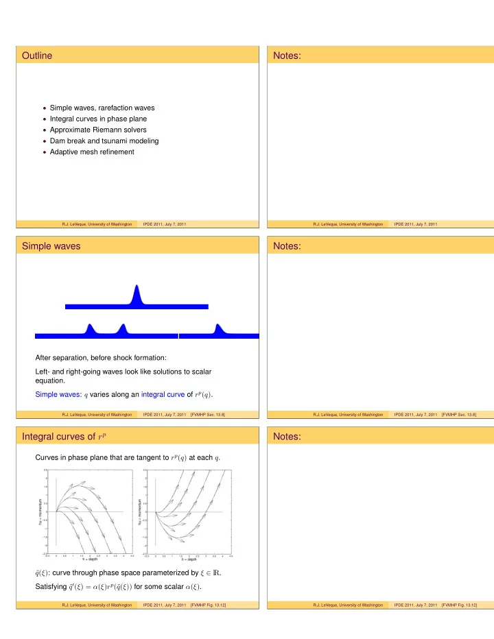
Integral curves of rp
Curves in phase plane that are tangent to rp(q) at each q. ˜ q(ξ): curve through phase space parameterized by ξ ∈ lR. Satisfying ˜ q′(ξ) = α(ξ)rp(˜ q(ξ)) for some scalar α(ξ).
R.J. LeVeque, University of Washington IPDE 2011, July 7, 2011 [FVMHP Fig. 13.12]
Notes:
R.J. LeVeque, University of Washington IPDE 2011, July 7, 2011 [FVMHP Fig. 13.12]