photon mapping

PhotonMapping e.g.refrac=onofacaus=c - PDF document

Refrac=onofaCaus=c MonteCarloraytracinghandlesall pathsoflight:L(D|S)*E,butnotequally well HasdifficultysamplingLS*DS*Epaths, PhotonMapping


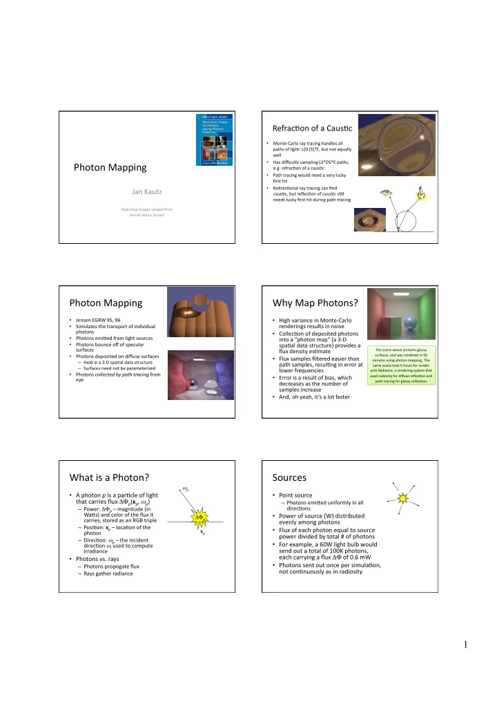
  1. Refrac=on
of
a
Caus=c
 • Monte‐Carlo
ray
tracing
handles
all
 paths
of
light:
L(D|S)*E,
but
not
equally
 well
 • Has
difficulty
sampling
LS*DS*E
paths,
 Photon
Mapping
 e.g.
refrac=on
of
a
caus=c
 • Path
tracing
would
need
a
very
lucky
 first
hit
 • Bidirec=onal
ray
tracing
can
find
 Jan
Kautz
 caus=c,
but
reflec=on
of
caus=c
s=ll
 needs
lucky
first
hit
during
path
tracing
 Featuring
images
swiped
from
 Henrik
Wann
Jensen
 Photon
Mapping
 Why
Map
Photons?
 • Jensen
EGRW
95,
96
 • High
variance
in
Monte‐Carlo
 renderings
results
in
noise
 • Simulates
the
transport
of
individual
 photons
 • Collec=on
of
deposited
photons
 • Photons
emiXed
from
light
sources
 into
a
“photon
map”
(a
3‐D
 • Photons
bounce
off
of
specular
 spa=al
data
structure)
provides
a
 surfaces
 flux
density
es=mate
 The
scene
above
contains
glossy
 surfaces,
and
was
rendered
in
50
 • Photons
deposited
on
diffuse
surfaces
 • Flux
samples
filtered
easier
than
 minutes
using
photon
mapping.
The
 – Held
in
a
3‐D
spa=al
data
structure
 path
samples,
resul=ng
in
error
at
 same
scene
took
6
hours
for
render
 – Surfaces
need
not
be
parameterized
 lower
frequencies
 with
Radiance,
a
rendering
system
that
 • Photons
 collected
by
path
tracing
 from
 used
radiosity
for
diffuse
reflec=on
and
 • Error
is
a
result
of
bias,
which
 eye
 path
tracing
for
glossy
reflec=on. 
 decreases
as
the
number
of
 samples
increase
 • And,
oh
yeah,
it’s
a
lot
faster
 What
is
a
Photon?
 Sources
 ω p • A
photon
 p 
is
a
par=cle
of
light
 • Point
source
 that
carries
flux
 ΔΦ p ( x p ,
 ω p )
 – Photons
emiXed
uniformly
in
all
 direc=ons
 – Power:
 ΔΦ p 
–
magnitude
(in
 WaXs)
and
color
of
the
flux
it
 • Power
of
source
(W)
distributed
 ΔΦ p carries,
stored
as
an
RGB
triple
 evenly
among
photons
 – Posi=on:
 x p 
–
loca=on
of
the
 • Flux
of
each
photon
equal
to
source
 x p photon
 power
divided
by
total
#
of
photons
 – Direc=on:
 ω p 
–
the
incident
 • For
example,
a
60W
light
bulb
would
 direc=on
 ω i 
used
to
compute
 send
out
a
total
of
100K
photons,
 irradiance
 each
carrying
a
flux
 ΔΦ 
of
0.6
mW
 • Photons
vs.
rays
 • Photons
sent
out
once
per
simula=on,
 – Photons
propogate
flux
 not
con=nuously
as
in
radiosity
 – Rays
gather
radiance
 1

  2. Mixed
Surfaces
 Russian
RouleXe
 ? • Surfaces
have
specular
and
 • Arvo
&
Kirk,
S90
 • Reflected
flux
only
a
frac=on
of
 diffuse
components
 ρ d = 50% incident
flux
 – 
 ρ d 
–
diffuse
reflectance
 ρ s = 30% • Aker
several
reflec=ons,
spending
 – 
 ρ s 
–
specular
reflectance
 a
lot
of
=me
keeping
track
of
very
 – 
 ρ d 
+
 ρ s 
<
1
(conserva=on
of
 liXle
flux
 energy)
 • Instead,
completely
absorb
some
 photons
and
completely
reflect
 • Let
 ζ 
be
a
uniform
random
value
 others

at
full
power
 from
0
to
1
 • Spend
=me
tracing
fewer
full
 • If
 ζ 
<
 ρ d 
then
reflect
diffuse
 power
photons
 • Else
if
 ζ 
<
 ρ d 
+
 ρ s 
then
reflect
 • Probability
of
reflectance
is
the
 reflectance
 ρ .
 specular
 • Probability
of
absorp=on
is
1
–
 ρ .

 ρ = 60% • Otherwise
absorb
 Storing
Photons
 K‐D
Tree
 • Uses
a
kd‐tree
–
a
sequence
of
axis‐ • Given
a
large
number
of
points
p 1 ,…,p n 
in
3D
 aligned
par==ons
 – 2‐D
par==ons
are
lines
 space
we
want
to
classify
them
and
be
able
to
 – 3‐D
par==ons
are
planes
 make
fast
queries:
 • Axis
of
par==ons
alternates
wrt
 depth
of
the
tree
 – Find
all
the
points
within
a
cuboid
 • Average
access
=me
is
 O (log
 n )
 – Find
all
the
points
within
a
neighbourhood
of
a
 • Worst
case
 O ( n )
when
tree
is
 severely
lopsided
 given
point
 • Need
to
maintain
a
balanced
tree,
 which
can
be
done
in
 O ( n 
log
 n )
 • These
points
are
photon
posi=ons
on
surfaces.
 • Can
find
k
nearest
neighbors
in
 O ( k 
+
log
 n )
=me
using
a
heap
 K‐D
Tree
 K‐D
Tree
 • A
K‐D
tree
is
just
an
axis
aligned
BSP
tree.
 • Write
p i 
=
(x 1i ,
x 2i ,
x 3i )
 • Let
x j *
be
the
median
of
the
values
of
the
jth
coordinate
 • Each
 node
 of
 the
 tree
 stores
 a
 separa=ng
 (j=1,2,3).
 • Start
with
x 1 *
which
will
par==on
the
original
set
of
points
 plane,
defined
by
the
median
value
along
one
 into
two
sets
(divided
along
the
X
axis).
 of
the
coordinates.

 • Now
apply
the
same
procedure
to
each
of
the
lek‐
and
right‐ sets,
except
now
subdivide
on
x 2 *

 • The
leaves
of
the
tree
contain
the
original
data
 • Now
apply
the
same
procedure
recursively
to
each
of
these
 points.

 subsets
except
now
subdivide
on
x 3 *

 • Keep
applying
this
recursively
un=l
each
leaf
of
the
tree
 contains
a
data
point.

 2

  3. K‐D
Tree
2D
Example
 K‐D
Tree
2D
Example
 K‐D
Tree
2D
Example
 K‐D
Tree
Code
 KDTree makeKDTree(int n, point_kd p[], int depth) /*returns a kd-tree for the n 3-dimensional points in p - assume all indices start from 1*/ { if n==1 return a leaf containing p[1]; /*base case*/ x = median of values of (depth mod 3) coordinate in the points; pLeft is the set of points to the left of x and pRight is the set to the right; leftNode = makeKDTree(n/2,pLeft,depth+1); rightNode = makeKDTree(n/2,pRight,depth+1); /*assumes that the median splits the points exactly in two*/ /*compose a new node and return*/ return compose(leftNode,x,rightNode); } K‐D
Tree
Advantages
 Reflected
Radiance
 • Using
a
K‐D
tree
solu=on
does
not
depend
on
 • Recall
the
reflected
radiance
equa=on
 the
 providing
 a
 mesh
 on
 the
 surfaces
 –
 the
 Δ A = π r 2 distribu=on
 of
 the
 photons
 is
 maintained
 • Convert
incident
radiance
into
incident
flux
 independently
 of
 the
 representa=on
 of
 the
 surfaces
 • The
method
does
not
rely
on
‘regular’
surfaces
 • Reflected
radiance
in
terms
of
incident
flux
 such
as
polygons,
but
could
equally
well
apply
 to
fractal
type
surfaces.
 • Numerically
 3

  4. How
Many
Photons?
 Filtering
 • How
big
is
the
disk
radius
 r ?
 • Too
few
photons
cause
blurry
 results
 • Large
enough
that
the
disk
 surrounds
the
 n 
nearest
 • Simple
averaging
produces
a
box
 photons.
 filtering
of
photons
 Radiance
es=mate
using
50
photons 
 • The
number
of
photons
used
for
 • Photons
nearer
to
the
sample
 a
radiance
es=mate
 n 
is
usually
 should
be
weighted
more
heavily
 between
50
and
500.
 • Results
in
a
cone
filtering
of
 photons
 Radiance
es=mate
using
500
 Δ A = π r 2 photons 
 Mul=ple
Photon
Maps
 Rendering
 • Rendered
by
glossy‐surface
 • Global
L(S|D)*D
photon
map
 distributed
ray
tracing
 – Photon
s=cks
to
diffuse
surface
 • When
ray
hits
first
diffuse
 and 
bounces
to
next
surface
(if
 surface…
 it
survives
Russian
rouleXe)
 – Compute
direct
illumina=on
 – Photons
don’t
s=ck
to
specular
 – Compute
reflected
radiance
 Caustic map Global map surfaces
 of
caus=c
map
photons
 First
diffuse
intersec=on.
 Use
global 
 photons photons Return
radiance
of
caus=c
 map 
 • Caus=c
LSS*D
photon
map
 – Ignore
global
map
photons
 map
photons
here,
but
 photons
to 
 – Importance
sample
BRDF
 f r 
 – High
resolu=on
 ignore
global
map
photons 
 return 
 as
usual 
 radiance 
 – Light
source
usually
emits
 – Use
global
photon
map
to
 when 
 photons
only
in
direc=ons
that
 importance
sample
incident
 evalua=ng 
 radiance
func=on
 L i
 hit
the
thing
crea=ng
the
caus=c
 Li
at
first 
 – Evaluate
reflectance
integral
 diffuse 
 by
cas=ng
rays
and
 intersec=on accumula=ng
radiances
from
 . 
 global
photon
map
 www.bennolan.com www.bennolan.com Examples
 Examples
 Direct
Illumina=on
 Global
Photon
Map
 4

Recommend


More recommend